Land Cover Change in the Andes of Southern  Ecuador—Patterns and Drivers

Curatola Fernández, Giulia F.; Obermeier, Wolfgang A.; Gerique, Andrés; López Sandoval, María Fernanda; Lehnert, Lukas W.; Thies, Boris; Bendix, Jörg

doi:10.3390/rs70302509

Open AccessArticle

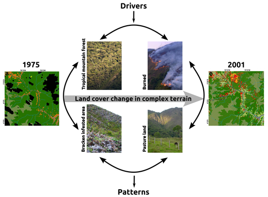
Land Cover Change in the Andes of Southern Ecuador—Patterns and Drivers

¹

Laboratory for Climatology and Remote Sensing, Faculty of Geography, University of Marburg, Deutschhausstr. 12, Marburg 35032, Germany

²

Institute of Geography, University of Erlangen-Nürnberg, Wetterkreuz 15, Erlangen 91058, Germany

³

Department of Development, Environment, and Territory, Latin American Faculty of Social Sciences—FLACSO Ecuador, Calle La Pradera E7-174 y Av. Diego de Almagro, Quito 170516, Ecuador

^*

Author to whom correspondence should be addressed.

Remote Sens. 2015, 7(3), 2509-2542; https://doi.org/10.3390/rs70302509

Submission received: 28 November 2014 / Revised: 7 February 2015 / Accepted: 17 February 2015 / Published: 3 March 2015

Download

Browse Figures

Versions Notes

Abstract

:

In the megadiverse tropical mountain forest in the Andes of southern Ecuador, a global biodiversity hotspot, the use of fire to clear land for cattle ranching is leading to the invasion of an aggressive weed, the bracken fern, which is threatening diversity and the provisioning of ecosystem services. To find sustainable land use options adapted to the local situation, a profound knowledge of the long-term spatiotemporal patterns of land cover change and its drivers is necessary, but hitherto lacking. The complex topography and the high cloud frequency make the use of remote sensing in this area a challenge. To deal with these conditions, we pursued specific pre-processing steps before classifying five Landsat scenes from 1975 to 2001. Then, we quantified land cover changes and habitat fragmentation, and we investigated landscape changes in relation to key spatial elements (altitude, slope, and distance from roads). Good classification results were obtained with overall accuracies ranging from 94.5% to 98.5% and Kappa statistics between 0.75 and 0.98. Forest was strongly fragmented due to the rapid expansion of the arable frontier and the even more rapid invasion by bracken. Unexpectedly, more bracken-infested areas were converted to pastures than vice versa, a practice that could alleviate pressure on forests if promoted. Road proximity was the most important spatial element determining forest loss, while for bracken the altitudinal range conditioned the degree of invasion in deforested areas. The annual deforestation rate changed notably between periods: ~1.5% from 1975 to 1987, ~0.8% from 1987 to 2000, and finally a very high rate of ~7.5% between 2000 and 2001. We explained these inconstant rates through some specific interrelated local and national political and socioeconomic drivers, namely land use policies, credit and tenure incentives, demography, and in particular, a severe national economic and bank crisis.

Keywords:

land cover change; remote sensing; Ecuador; Andes; fragmentation; bracken fern; deforestation drivers; Landsat; image pre-processing; attractors of landscape change

Graphical Abstract

1. Introduction

Human-induced land cover change is a threat to biodiversity and ecosystem services [1], particularly in biodiversity hotspots of the tropics [2,3,4]. Here, land cover change dynamics are extremely diverse and intricate because they depend strongly on complex regional interactions between people and the specific environment [5], crosscutting local to global scales [6,7]. Therefore, the patterns and pace of local land cover change are difficult to deduce from broader scales or from other local studies, even in the same country [8].

In Ecuador, most of the studies have focused on the Amazonian lowlands [9,10,11,12,13,14,15,16,17,18,19,20,21,22] and coastal [5,8,23,24] regions, while land cover change in the Andes has been studied less, due, among other reasons, to the inaccessibility of the region. It is obvious that in remote areas like the Ecuadorian Andes, wide analysis of land cover change would not be possible without the use of remotely sensed data. However, the topographical complexity in such locations and particularly the high cloud frequency of the Andes makes the use of remote sensing techniques a challenge [25,26,27]. Accurate atmospheric and topographic corrections of the satellite scenes are a prerequisite to obtain satisfactory classification results [25,28,29,30,31,32], but are not always performed due to time and resource limitations [33].

In the San Francisco Valley breaching the south-eastern Ecuadorian Andes and its surroundings (refer to Section 2.1), large areas of tropical mountain forest have been cleared, mostly for agricultural expansion of smallholder cattle-ranching [34,35,36,37,38,39]. Since 2002, this location has been the subject of two consecutive multidisciplinary projects that have been investigating the ecosystem functioning and services for sustainable land use management [38,40]. However, previous research only focused on particular subjects related to land cover and land cover change, with some of them relying only on analysis of one or a few satellite images covering short time periods. These few studies revealed a high degree of deforestation related to topography and road infrastructure [35,41,42]. Other socioeconomic studies from this area found a strong relationship between land cover change and private land tenure systems, cattle ranching, and decrease of local traditional ecological knowledge on plant use [34,36,43]. Moreover, a recurrent problem recognized in all the studies is the invasion of bracken fern (Pteridium arachnoideum and Pteridium caudatum), a fire-resistant and very competitive weed [38,44,45,46] that colonizes unused burnt or inactive pasture areas, or even active pastures [44,45,46]. Bracken invasion frequently leads to pasture abandonment, which takes the area out of the production process, degrades ecosystem functions and services, and threatens the remaining natural forest [47]. Possible solutions for avoiding deforestation in the study area have been explored by means of payment schemes that include productive land use concepts [48].

Despite the knowledge hitherto gained, a comprehensive approach to study land cover change in the SE-Ecuadorian Andes over an extended period considering fragmentation, fire–pasture–bracken dynamics, and the study of proximate and local and non-local underlying drivers is still lacking.

Landsat data, with its spatial resolution of 30–60 m, longer term (since 1972), and free availability, is especially suitable for land cover change detection, as already demonstrated elsewhere in a variety of studies [49,50,51,52,53]. Due to the complex terrain and the difficult weather conditions in the study area, an accurate change detection analysis is only possible if an adequate atmospheric and topographic correction is applied to the satellite images. Additionally, other pre-processing steps like (i) image co-registration; (ii) cloud/cloud-shadow detection; and (iii) intercalibration are also necessary to produce accurate results. Hence, a framework to conduct the required processing steps with a minimum of manual work is needed to fully exploit this valuable source of information efficiently.

Consequently, the main aims of this paper are (i) the development and implementation of a semi-automated processing framework to allow an accurate classification of Landsat scenes in complex terrain; and, based on this, (ii) to present an integrated view of the land cover change process in the Upper Zamora and San Francisco Valleys from 1975 until 2001. The results of this study are fundamental for the ongoing research in this region, particularly to identify other potential alternatives of sustainable land management adapted to the geographical, ecological, cultural, and historical reality [54,55,56,57]. Moreover, the development of the pre-processing tool for the Landsat scenes is of benefit not only for future monitoring of the land cover change in this area but also for research on land cover change in tropical mountain forests in general.

2. Study Area

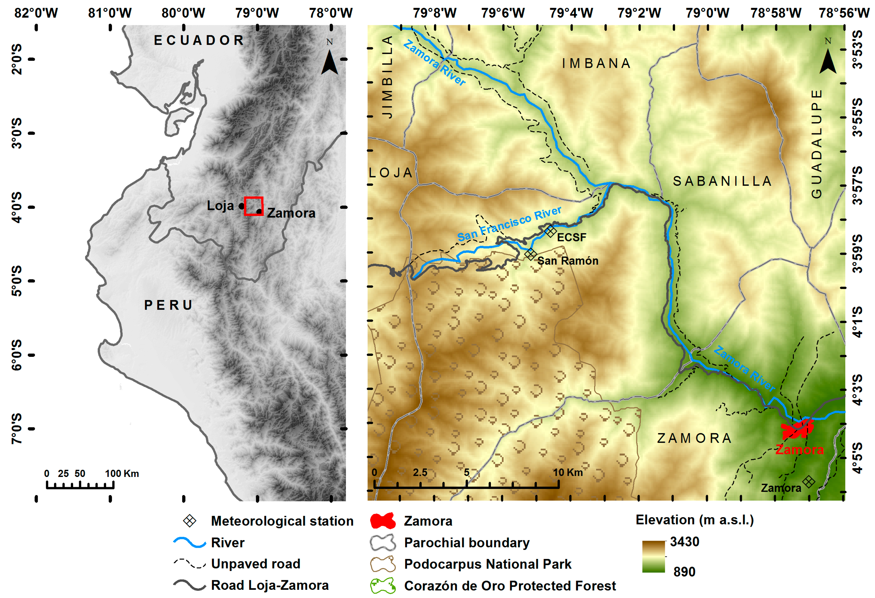
2.1. Geographical Setting

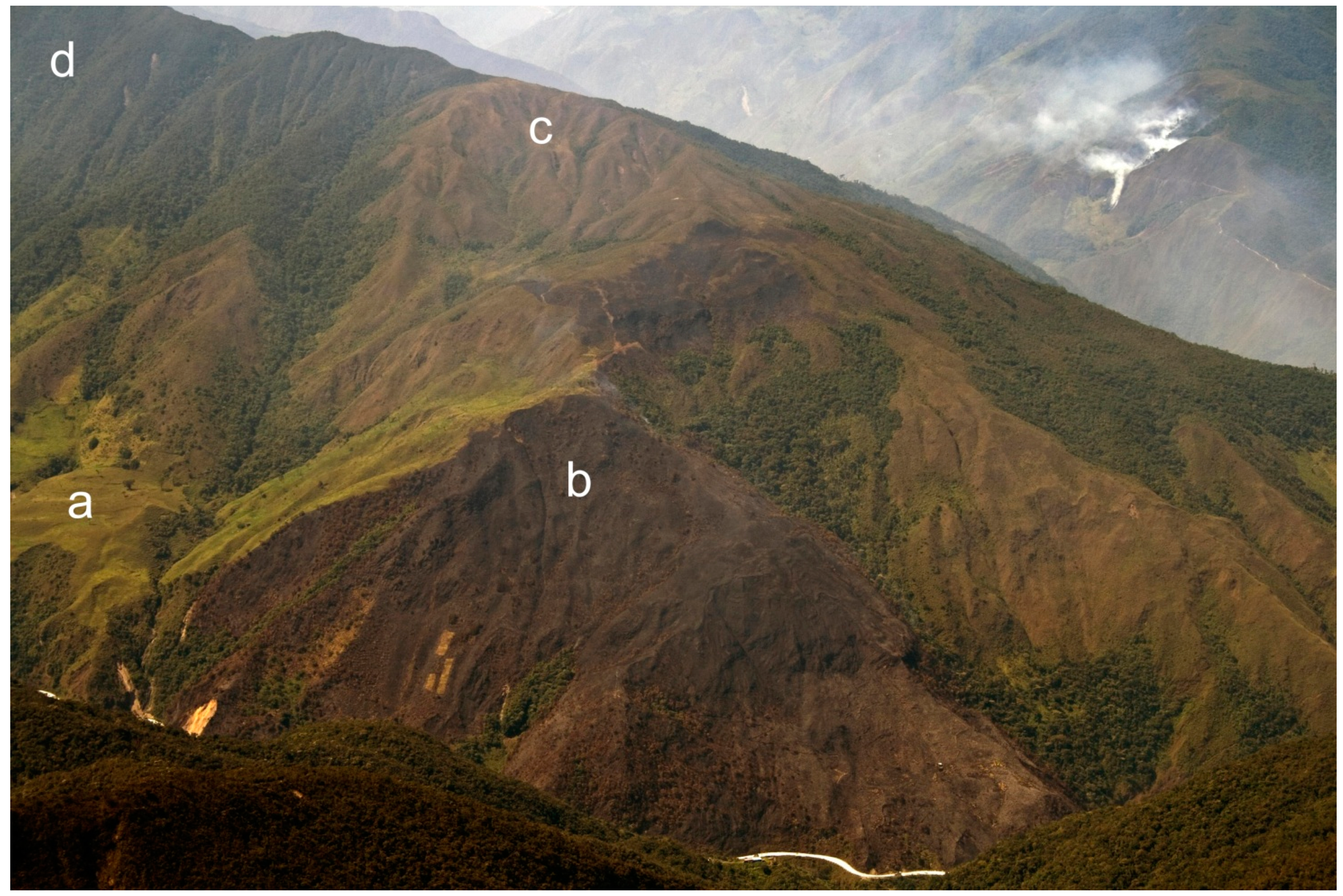
The study area (~25 by 25 km) is located at the eastern slopes of the South Ecuadorian Andes in the Huancabamba depression, a region where the Andes are comparatively lower in elevation but with a higher topographical complexity (Figure 1). This complexity and the strong altitudinal gradient from ~900 to ~3500 m above sea level (a.s.l.) result in a high heterogeneity of environmental conditions, among others, leading to an outstanding diversity of vascular plants [58] and other organisms, mostly harbored by the natural mountain rain forest [38,40]. The region has a tropical humid climate with an extremely wet period from April to July and a relatively dry period from September to December [59]. According to Homeier et al. [60], the forest upper boundary reaches an altitude of ~2700 m a.s.l., where it is replaced by subpáramo and páramo vegetation. Since 1982, the southwestern part of the study area has belonged to the Podocarpus National Park, and since 2000 the northern part has belonged to the Corazón de Oro Protected Forest.

Figure 1. Study area embedded in the Andes of southern Ecuador (left) with a detailed view corresponding to the extension of the analyzed satellite data (right).

Politically, the area under investigation comprises the rural parishes (parroquias) of Imbana, Sabanilla, and Zamora in the Zamora-Chinchipe province, where most of the inhabitants are Mestizo settlers (~80%, [61]). The northern part of the study area has been mainly colonized by the Saraguros, a Quechua indigenous group from the highlands of Loja province. The main road crossing the area connects Loja (capital of the Loja province) and Zamora (capital of the Zamora-Chinchipe province).

2.2. Land Use

The cultural landscape in the study area is principally composed of a mosaic of forest patches, pastures, and bracken-infested areas (Figure 2), the latter being a less diverse and probably long-lasting system [39,44].

New pastures are established for three main reasons: (i) to counterbalance the fertility loss of old paddocks with low stock rates; (ii) to increase production [8]; and (iii) because of the invasion of bracken fern (Pteridium arachnoideum and Pteridium caudatum) [43,44,45].

As in similar areas of Latin America [62], slash and burn is the traditional way of establishing and rejuvenating pastures. After choosing an area of about one hectare, the inhabitants remove high value forest timber species [37]. During the beginning of the dry period, they cut parts of the understory and the remaining trees, let the area dry out, and burn the plot [37]. Normally, fire stops at the plot edge, as forest moisture inhibits its passage. However, strong winds, dry periods, the presence of neighboring dry bracken-infested areas [39], or/and the use of fire accelerators can lead to burning adjacent forest areas [37]. The clearing of more land than farmers can hold under use (due to labor scarcity or other household factors) leads to the establishment of bracken-dominated vegetation [37], mostly found in the steepest areas [34,36]. Once the soil cools down, farmers quickly plant pasture grasses, given that about three weeks after fire bracken fern sprouts vigorously [45]. If the emerging bracken sprouts are not eliminated, they will expand, making their eradication very time-consuming and labor-intensive [63].

Figure 2. Landscape in the San Francisco River Valley during the dry season: (a) pastures; (b) recently burned areas; (c) bracken-infested area; and (d) forest (Photograph by Sandro Makowski Giannoni, October 2010).

3. Methods

As stressed in the introduction, atmospheric and topographic corrections and other pre-processing steps are a fundamental prerequisite to obtain satisfactory classification results for land cover change studies in regions of complex terrain. Because of the high amount of data and time and resource limitations, a semi-automated processing chain with a minimum of manual intervention was developed. In the following sections, we present a description of the pre-processing steps (3.1), the image classification (3.2), and the change detection analysis (3.3 and 3.4).

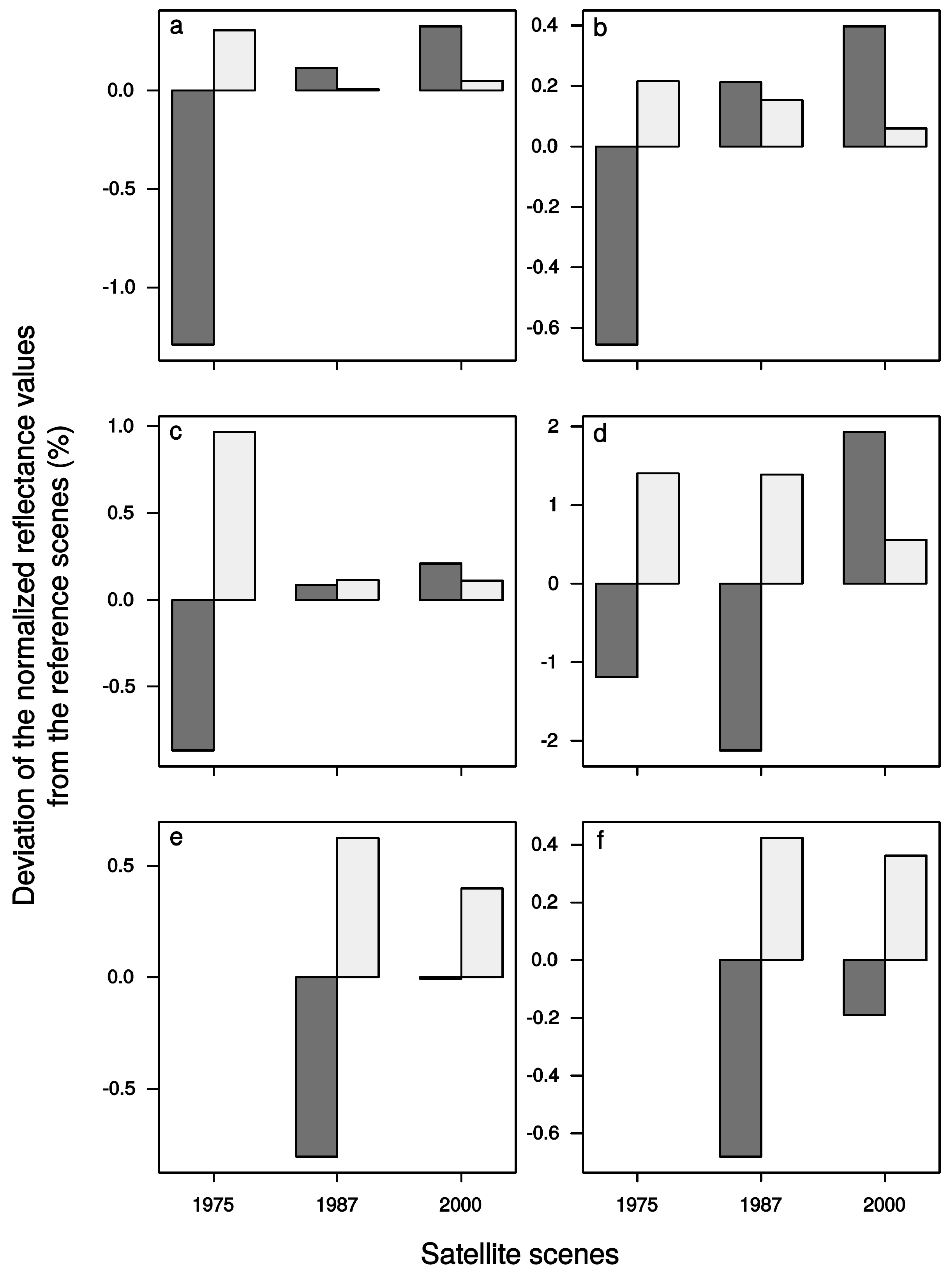
3.1. Pre-Processing of Landsat Scenes

We chose all available Landsat satellite images for the study area from the United States Geological Survey (USGS) website [64] which had less than 50% cloud cover and no data gaps originating from the failure of the system’s scan line corrector (SLC) of Landsat ETM+. Our intention was to cover the longest attainable time period. This resulted in five images covering the period from 1975 to 2001 (Table 1).

Table 1. Satellite data used.

**Table 1.** Satellite data used.
Date	Satellite	Sensor	Spatial Resolution (m)	Spectral Bands	Cloud Cover (%)
28 December 1975	Landsat 2	MSS	60	2 visible, NIR	7.9
19 December 1980	Landsat 2	MSS	60	2 visible, NIR	12.0
26 March 1987	Landsat 5	TM	30	3 visible, 2 NIR, MIR	24.1
31 October 2000	Landsat 7	ETM+	30	3 visible, 2 NIR, MIR	41.1
3 November 2001	Landsat 7	ETM+	30	3 visible, 2 NIR, MIR	0.0

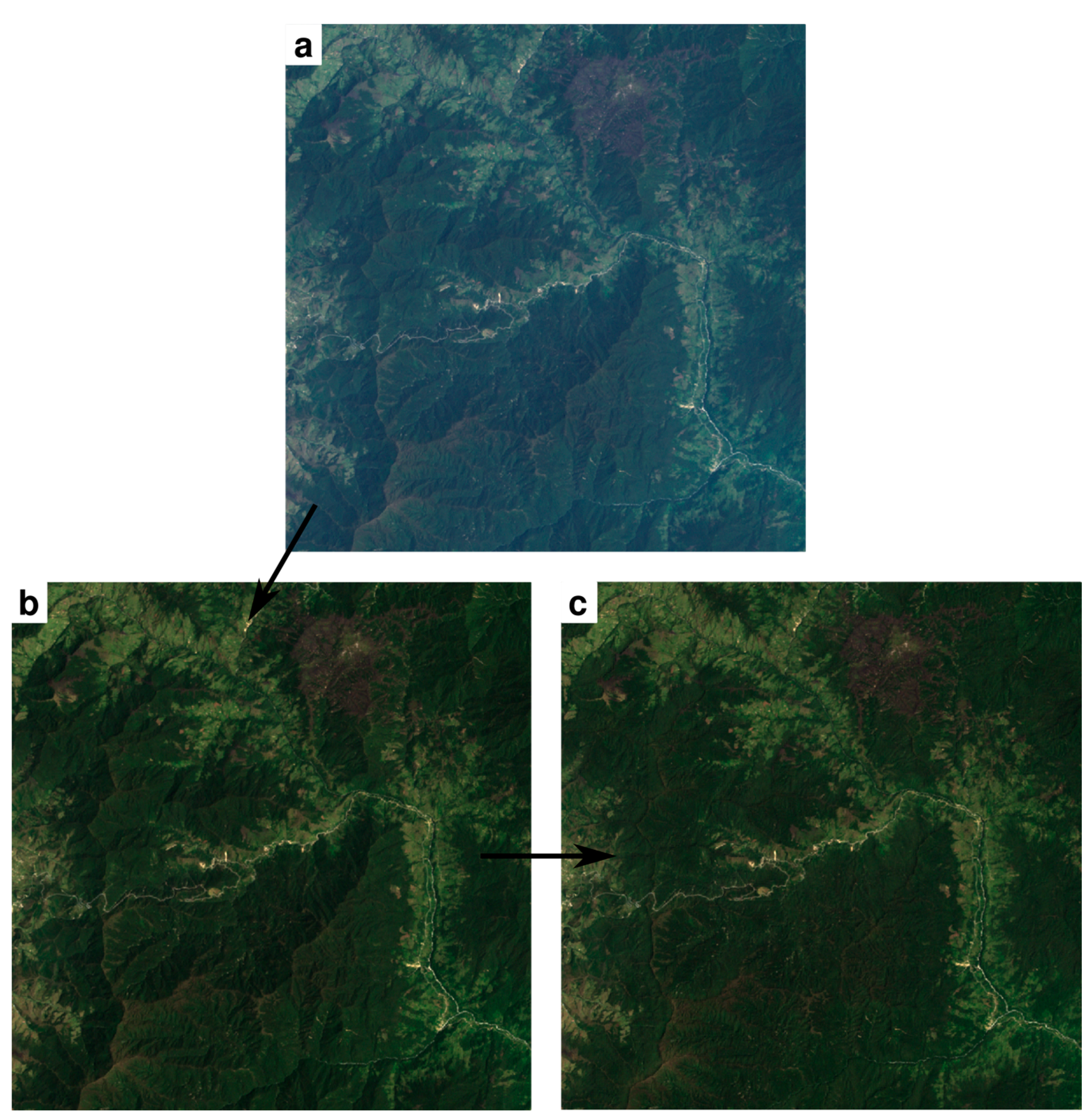
3.1.1. Co-Registration

For spatial accuracy of change detection, the satellite images were co-registered to one reference image (2001) using the first-order polynomial function. Root mean square errors of less than half a pixel were achieved for all images.

3.1.2. Masking Clouds and Cloud-Shadows

Cloud and cloud-shadow masks were developed for the four scenes with cloud cover (Table 1). The cloud and cloud-shadow mask of the scene from 1980 was digitized directly from a false color RGB composite due to the presence of only a few isolated clouds. For the other three cloud-contaminated scenes, we adapted the method of Martinuzzi et al. [27]. First clouds were identified by classifying band 1 (or 4 in the case of Landsat MSS) and 6 (thermal band only available in Landsat TM and ETM+) using digital number (DN) brightness ranges (Table 2). Each classification was buffered to assure a complete inclusion of the clouded areas. In the case of Landsat TM and ETM+, the cloud mask resulted from the intersection of both classifications, since the cloud classification of band 1 included bare soil and some urban regions and the cloud classification of band 6 included dense forested areas. Due to the lack of the thermal band in the MSS scene, we visually corrected the cloud classification of band 4. Additionally, a buffer was applied to the cloud masks. Afterwards, cloud-shadow masks were created by shifting the cloud masks over the cloud-shadowed surfaces using the nearest neighbor algorithm. For this, cloud-shadows were identified in band 4 (or 7 for Landsat MSS) and distinctive points both in the cloud mask and cloud shadows were selected. Then, the cloud and cloud-shadow masks were combined and a further buffer was applied to remove remaining cloud-shadow-contaminated pixels originating from topographic distortions. The final cloud and cloud-shadow masks were manually inspected and corrected.

Table 2. Digital number (DN) brightness ranges and buffer size for the cloud and cloud-shadow masking. Band 1 corresponds to the Landsat TM scenes of 1987 and 2000, and band 4 corresponds to the Landsat MSS scene of 1975.

**Table 2.** Digital number (DN) brightness ranges and buffer size for the cloud and cloud-shadow masking. Band 1 corresponds to the Landsat TM scenes of 1987 and 2000, and band 4 corresponds to the Landsat MSS scene of 1975.
	DN Brightness Range		Buffer (Pixels)
Scene	Band 1 (or 4)	Band 6	Mask Band 1 (or 4)	Mask Band 6	Cloud Mask	Cloud Mask + Cloud-Shadow Mask
1975	29–127		2		2	10
1987	83–256	91–256	3	4	2	4
2000	87–256	82–256	6	4	3	10

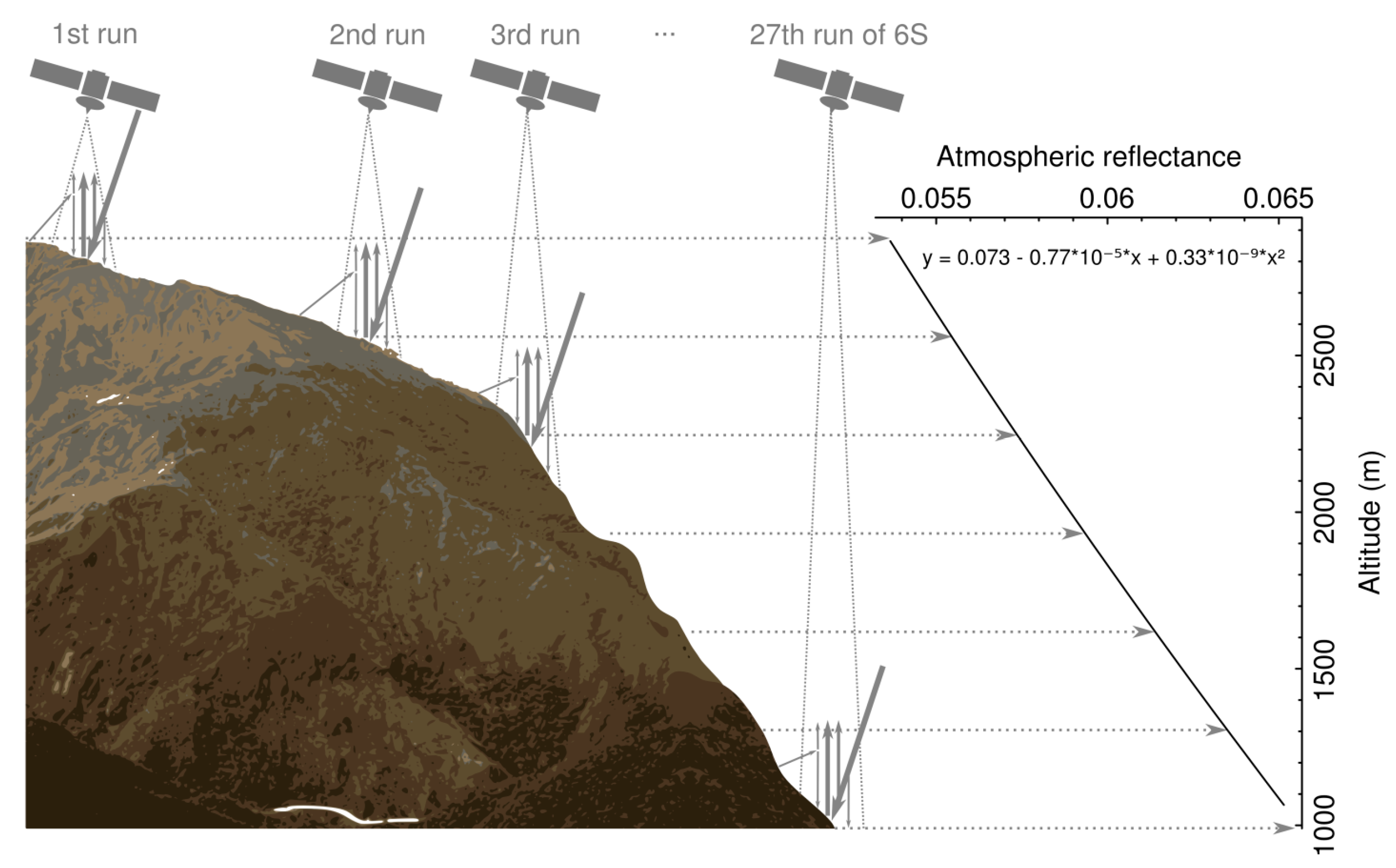
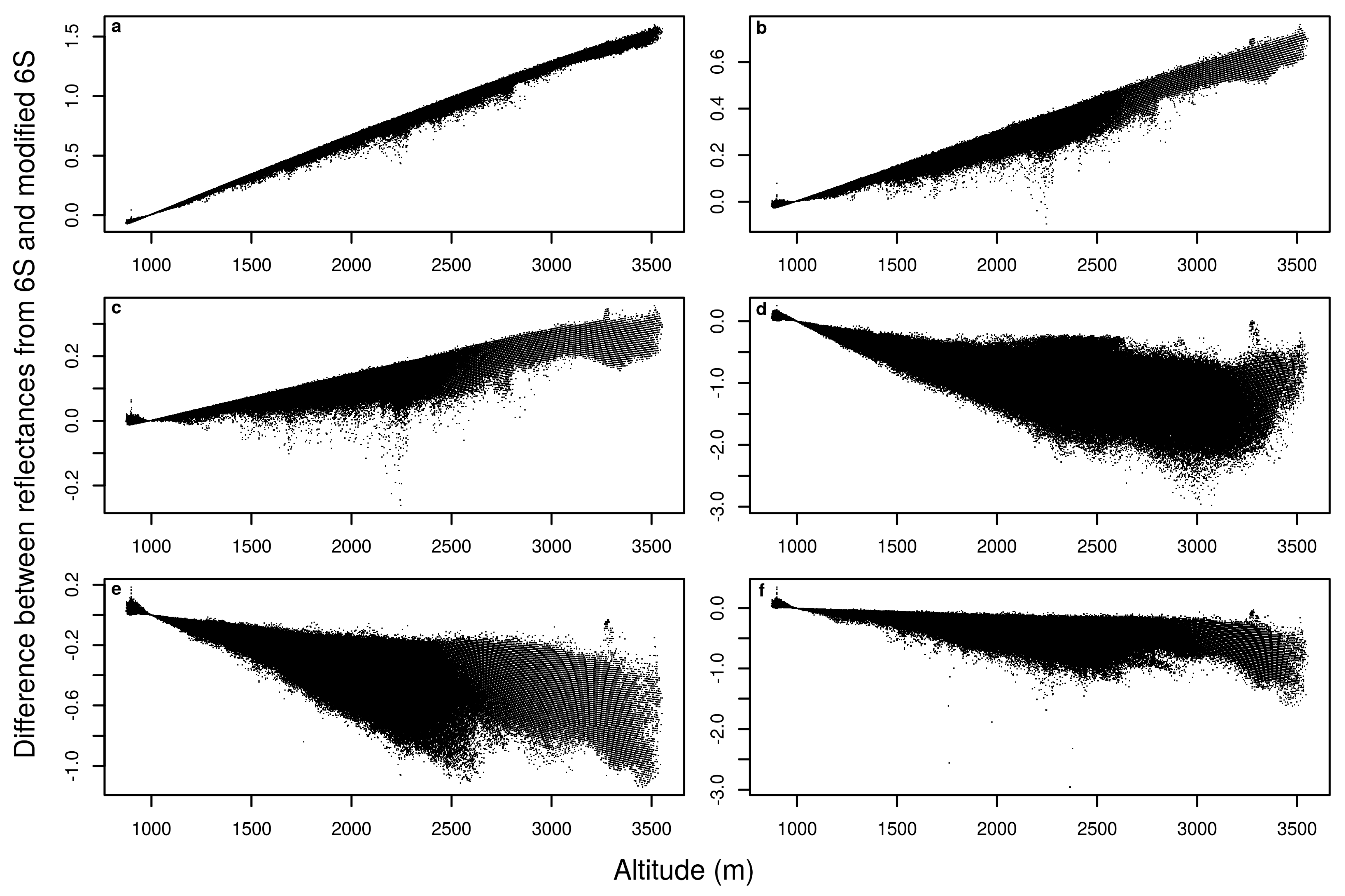
3.1.3. Atmospheric and Topographic Correction

To compensate for the varying atmospheric effects within the study area, we developed a fully automatic module (AtToCor) combining an extended version of the Second Simulation of the Satellite Signal in the Solar Spectrum radiative transfer code (6S code [65]) and a topographic correction module.

In order to apply the 6S code for area-wide and automatic operation, two modifications are implemented in AtToCor: (i) an area-wide adaptation to highly variable terrain altitudes; and (ii) an automatic scheme to consider an as-exact-as-possible representation of the atmosphere over the area of interest for the time of image acquisition.

(i) In the original version of the 6S code, the atmospheric absorption, reflection, and scattering coefficients are calculated for one single altitude. In the modified version, the parameters are calculated for 27 altitude levels spanning the entire range of the terrain in the respective satellite image (Figure 3). The 27 parameters are then used to estimate the effect of the altitude on each parameter by fitting second-order polynomial regression models between atmospheric absorption, reflectance, and scattering coefficients and altitude. The number of altitude levels was set to 27 to ensure a sufficiently high number of samples to train the polynomial regression models. This approach allows for the estimation of atmospheric effects in relation to the pixel’s altitude from a co-located digital elevation model.

Figure 3. (Left) Schematic overview of the atmospheric absorption, transmittance, and reflectance calculated in the modified version of the 6S code for 27 altitudinal layers. (Right) As an example, we plotted the atmospheric reflectance regression line of band 1 of the Landsat ETM+ scene of 2001 according to the elevation.

(ii) The atmospheric pressure, water vapor, and temperature profiles in the original 6S version either rely on values of standard atmosphere or require data from radiosondes, which are mostly unavailable outside the industrialized countries, and not in mainland Ecuador. We implemented the option to extract and download the profiles of air temperature and specific humidity at different pressure levels for the over-flight day automatically from reanalysis data [66] at the National Center for Environmental Prediction/National Center of Atmospheric Research (NCEP/NCAR) website [67] (Table 3). Using the center location of the image and the time of acquisition, the profiles are temporarily and spatially interpolated.

Table 3. Atmospheric composition at time of image acquisition. Missing values (NA) were filled with the tropical standard atmosphere values from the Second Simulation of the Satellite Signal in the Solar Spectrum radiative transfer code (6S code).

**Table 3.** Atmospheric composition at time of image acquisition. Missing values (NA) were filled with the tropical standard atmosphere values from the Second Simulation of the Satellite Signal in the Solar Spectrum radiative transfer code (6S code).
	1975		1980		1987		2000		2001
Tot. column Ozone (Dobson Unit)	NA		250		243		240		265
Visibility (km)	30.56		30.56		31.25		34.45		35.58
	Air temp.	Spec. hum.	Air temp.	Spec. hum.	Air Temp.	Spec. hum.	Air temp.	Spec. hum.	Air Temp.	Spec. hum.
Pressure level (Pa)	(K)		(K)		(K)		(K)		(K)
1000	296.2	0.01378	296.7	0.01492	300.1	0.01998	295.8	0.01282	295.8	0.01247
925	291.8	0.01131	292.3	0.01226	296.0	0.01679	292.3	0.01115	292.4	0.01088
850	288.1	0.00987	288.5	0.01170	291.1	0.01373	288.8	0.01020	288.8	0.01067
700	281.0	0.00672	281.6	0.00827	281.9	0.00730	280.9	0.00834	282.9	0.00447
600	274.1	0.00539	274.5	0.00348	276.5	0.00391	275.6	0.00396	277.1	0.00192
500	266.2	0.00280	267.7	0.00283	268.8	0.00229	268.4	0.00074	268.4	0.00085
400	255.8	0.00003	259.4	0.00011	258.2	0.00164	257.9	0.00012	257.6	0.00033
300	239.4	0.00043	241.5	0.00017	243.4	0.00050	242.0	0.00003	240.7	0.00003
250	229.8	NA	231.7	NA	232.9	NA	232.4	NA	231.2	NA
200	218.7	NA	222.2	NA	221.7	NA	220.0	NA	221.4	NA
150	205.6	NA	207.2	NA	207.6	NA	205.3	NA	208.5	NA
100	194.6	NA	198.4	NA	194.2	NA	194.3	NA	194.5	NA
70	200.1	NA	199.2	NA	195.2	NA	196.0	NA	198.8	NA
50	210.4	NA	207.6	NA	203.7	NA	206.1	NA	208.1	NA
30	216.6	NA	215.0	NA	216.6	NA	209.9	NA	214.4	NA
20	221.7	NA	222.1	NA	222.0	NA	217.1	NA	221.0	NA
10	229.2	NA	230.7	NA	235.8	NA	234.8	NA	235.0	NA

The 6S code requires the proper definition of several other parameters for the conversion of top-of-atmosphere radiance values into at-surface reflectance values. We relied on the information of the sun–sensor–soil geometry (extracted automatically from the metadata of the scenes), on the atmospheric ozone content data and horizontal visibility, and on topographic variables. The total column ozone content value at the time of image acquisition is automatically extracted and downloaded to AtToCor from the Total Ozone Mapping Spectrometer (TOMS) satellite data [68]. Horizontal visibility was manually determined using data from a scatterometer installed in 2002 at a meteorological station in the study area [59]. For imagery acquired before 2002, we used monthly averages of the observation period 2002–2007. Topographic variables were derived from a digital elevation model (DEM) from the Shuttle Radar Topography Mission 3 (90 m resolution), which was bilinearly resampled to the resolution of the satellite imagery.

To test the importance of the factor terrain altitude for the atmospheric correction, we ran the original and the modified version of the 6S code with the bands of the Landsat ETM+ scene of 2001. We then compared the reflectance values of the bands corrected with these two modes.

To compensate for illumination effects arising from the rugged topography in our study area after the atmospheric correction, a topographic correction based on correlations between illumination and reflectance values was applied [69]. We used a semi-empirical approach, which first establishes a linear regression model between reflectance values and illumination. The corrected reflectance values are then calculated by subtracting the illumination effect estimated by the linear model from the uncorrected reflectance values derived by the 6S code.

3.1.4. Radiometric Intercalibration

To use the same spectral signatures for the selected land cover classes (see Table 4) in different years and for different sensors, the satellite scenes were radiometrically normalized (or intercalibrated). A straightforward regression method was applied [70], which uses the least squares of all pixels of one band to calculate normalization coefficients. It is based on the assumption that stable land cover types should have the same spectral signals in different images [71]. The accuracy of this method depends on the accuracy of the images’ co-registration, as well as on the absence of significant reflectance changes between the scenes [72], such as changes in vegetation phenology [73]. Since the image co-registration performed well (i.e., the root mean square error was smaller than half a pixel) and changes in phenology do not play an important role in tropical evergreen mountain forests, we considered the regression method suitable for our case. We used the scene of 2001 as a reference for the correction of the TM and ETM+ imagery, and the scene of 1980 to correct the MSS scene of 1975. To evaluate the accuracy of this method we selected a subset of forest that was assumed to have not significantly changed during the observation period and we compared the deviation of the normalized reflectance values from the reference scenes before and after the intercalibration (Figure 4). In general, the intercalibration reduced the difference of reflectance between the scenes, improving the comparability among them. No improvement was noticed in the red bands of the scenes of 1975 and 1987 (Figure 4c), in the NIR band of the scene of 1975 (Figure 4d), or in the MIR bands of the scene of 2000 (Figure 4e–f).

Table 4. Land cover classes.

**Table 4.** Land cover classes.
Land Cover Class	Description
Forest	All primary and secondary forest types
Pasture	Mainly Setaria sphacelata, Melinis minutiflora, Axonopus compressus, Pennisetum clandestinum, and Holcus lanatus
Bracken fern	Bracken fern and a mixture of other pioneer species
Non-vegetated	Roads, buildings, landslides, and bare soil
Water	Lakes and rivers
Burnt	Areas affected by a recent burning event
Mask	Clouds, cloud-shadows, and areas covered by subpáramo vegetation

Figure 4. Deviation of the normalized reflectances from the reference scenes (1980 and 2001) for a no-change subset of forest, before (dark bars) and after (bright bars) the intercalibration, in the (a) blue; (b) green; (c) red; (d,e) NIR 1 & 2; and (f) MIR bands of the Landsat satellite images of 1975, 1987, and 2000.

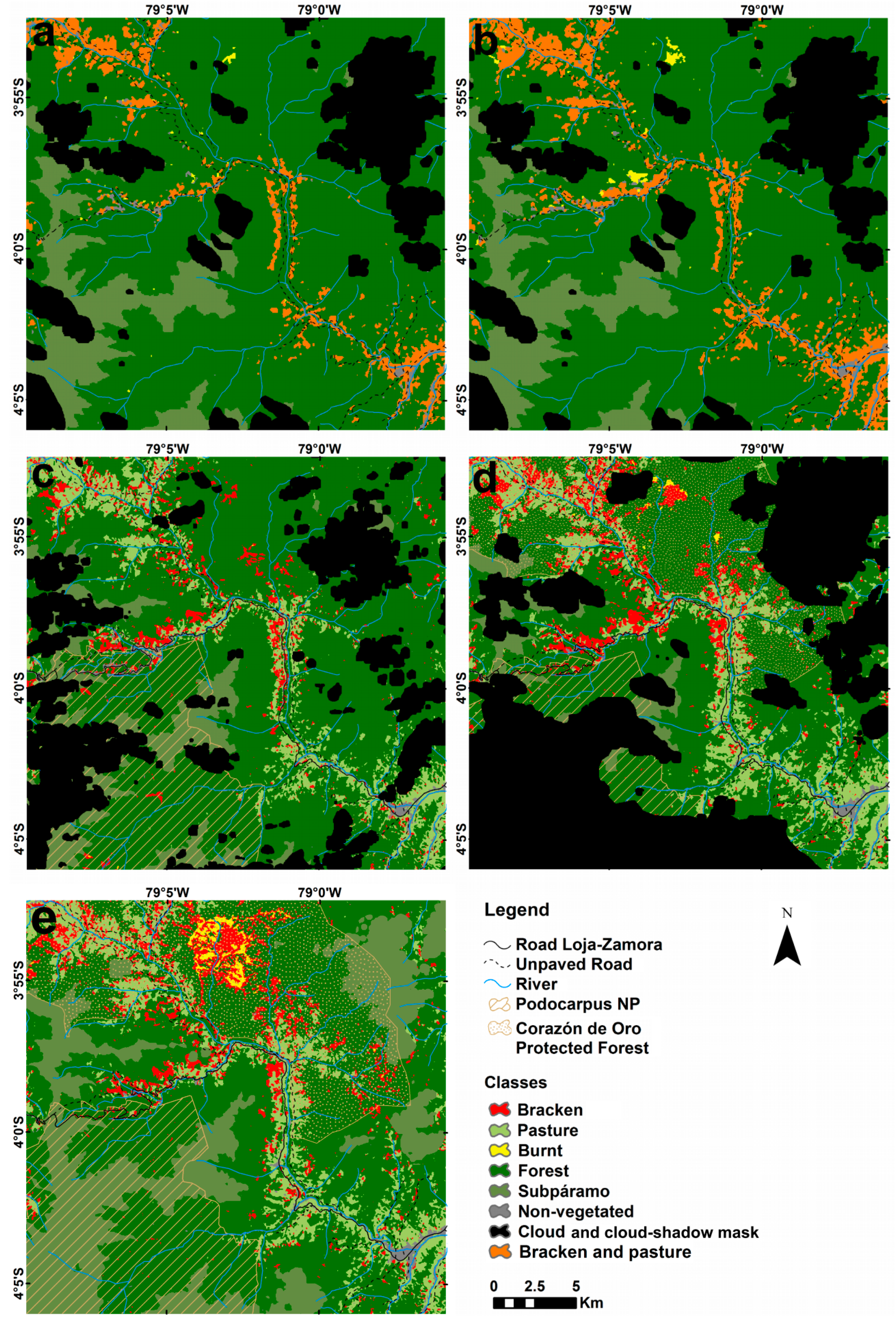
3.2. Land Cover Classification

Prior to the classification, the area above 2700 m a.s.l. was masked out. This altitude is covered by subpáramo [60], which presents low human impact and a spectral signal similar to bracken–infested areas. Then, spectral signatures were extracted from training sites in the reference scenes of 2001 and 1980 for the land cover classes presented in Table 4. Due to the coarser spatial and spectral resolution of MSS scenes and the unavailability of ancillary data for image interpretation, only four classes were separated in the two oldest scenes: “forest”, “pasture and bracken”, “non-vegetated”, and “water”.

Training sites in the Landsat ETM+ image of 2001 were selected based on expert knowledge and visual interpretation of an ortho-photograph mosaic (1 m resolution), derived from several flights in 2001 and processed by aero-triangulation techniques (aerial photograph: [74]; training sites: [35]). Generally, a sample size 10 times higher than the number of bands is recommended to account for the spectral variability within each of the classes [75]; given the use of six bands, we collected between 70 and 409 training pixels for each class. Training sites for the scene of 1980 were collected only by satellite image interpretation because no auxiliary data taken at the time of image acquisition were available. False RGB composites were generated to enhance the contrast between different land covers and to facilitate visual interpretation. Additionally, we overlaid the RGB composite images of the other years to compare possible land cover changes as a further interpretation aid. Given that Landsat MSS has four bands, we collected between 43 and 341 training pixels. The spectral signatures of the land cover classes generated from the training sites of the 2001 scene were also used for classifying the 2000 and 1987 scenes. Likewise, the signatures extracted from the 1980 scene were also used for the classification of the 1975 scene.

The maximum likelihood classification (MLC) approach was applied because it was already successfully used for other Landsat classifications in the study area [35,41,42]. Moreover, for classification approaches in the Brazilian Amazon based on Landsat data, MLC has been found to outperform new methods such as the artificial neural networks and classification tree [76]. After classification, the class “water” was merged with the class “non-vegetated.”

The accuracy of the classification results was assessed by compiling a contingency matrix and calculating the kappa index of agreement [77,78]. Validation sites in the image of 2001 were selected based on expert knowledge and visual interpretation of the ortho-photograph mosaic (as mentioned above for the training sites collection). For all the other scenes (2000, 1987, 1980, and 1975), validation sites were selected based on visual interpretation of the RGB composites of each year. None of the validation sites were used to train the MLC.

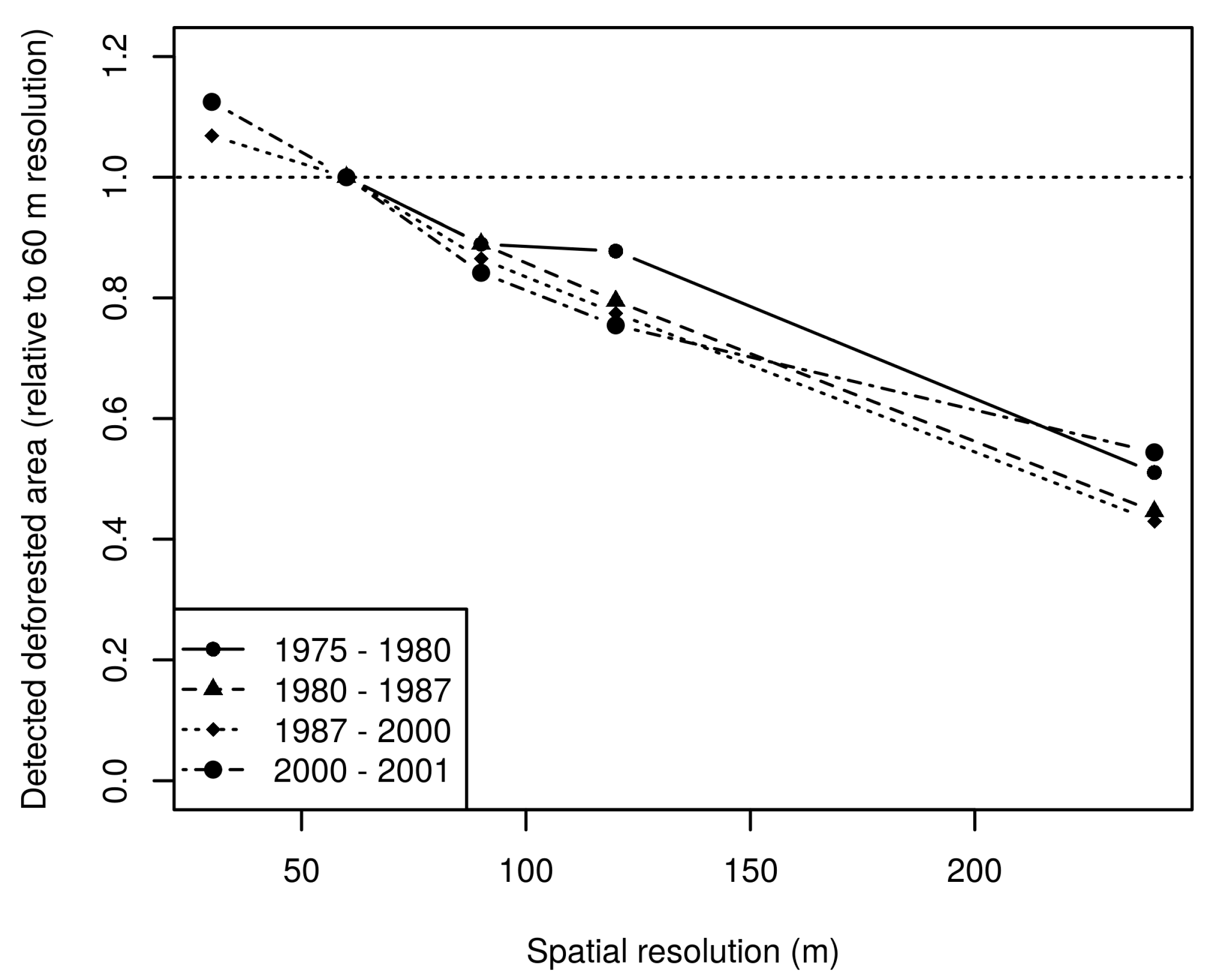
3.3. Quantification of Land Cover Change and Habitat Fragmentation

We quantified land cover change by means of the post-classification inter-comparison technique, nowadays one of the most used change detection approaches [79]. It implies a pixel-by-pixel comparison of separately classified images where the same cell size is required. We resampled the two coarse resolution maps of 60 m to 30 m using the nearest neighbor algorithm to avoid information loss in the three fine spatial resolution maps. This procedure has been found to perform similarly to the resampling method, which coarsens the fine resolution map [79].

The proportion of transition between the periods 1975–1980, 1980–1987, 1987–2000, and 2000–2001 was calculated using the following formula:

P_ij = (S_ij(t₁)/S_i(t₀)) × 100

(1)

where P_ij is the proportion of transition from class “i” to class “j”, S_i(t₀) is the surface of the “i” element of the transition matrix for the initial year, and S_ij(t₁) is the surface of the matrix element “ij” in the following time step.

Annual rates of deforestation (r) were calculated as well, using the following formula [14,16]:

r = 1 − {1 − [(A₁ − A₂)/A₁]}^1/t × 100

(2)

where A₁ and A₂ are the forest areas at the beginning and end of a given time period, and t is the number of years in that time period.

From an ecological perspective, the investigation of change rates and their reasons is not sufficient. Knowledge of habitat fragmentation in the natural system is fundamental for a better understanding of the ecological consequences, such as biodiversity loss, threat by e.g., invasive species, habitat decline, and climate change [80,81,82]. To detect habitat fragmentation in the different scenes, we used the program Fragstats [83]. We calculated the number of patches and the mean patch size of the main land cover classes (forest, pasture, and bracken), as both parameters are considered excellent indicators of landscape fragmentation [84,85].

The use of multiresolution imagery for land cover change detection can result in a bias. For each of the four abovementioned periods (1975–1980, 1980–1987, 1987–2000, and 2000–2001), this bias was estimated by consecutively reducing the spatial resolution to 60, 90, 120, and 240 m and to 90, 120, and 240 m for the imagery with the higher and the lower spatial resolution, respectively. The nearest neighbor resampling method was applied for resolution reduction. At each of the resolutions, the size of the deforested area was counted.

3.4. Analysis of Land Cover Change in Relation to Distance from Roads, Altitude, and Slope

Land cover change does not occur homogeneously in space. Certain site conditions or adjacency relationships—also called attractors of landscape change—result in some areas changing more rapidly than others [55].

Following the findings of Goerner et al. [41], Göttlicher et al. [35], and Thies et al. [42], we considered the distance from roads, altitude, and slope as the most important attractors of landscape change in our study area. Different studies have shown that the more easily reachable a forest is (close to roads and/or at lower altitude and/or slope), the higher the possibility of it being disturbed [86,87,88].

We quantified the annual land cover changes of forest, pasture, and bracken-infested areas in relation to these three attractors. Altitude and slope were obtained from the DEM and a roads vector file of the province of Zamora-Chinchipe was acquired from the Instituto Geográfico Militar del Ecuador (IGM) and adapted to historical state using the Landsat scenes.

4. Results and Discussion

4.1. AtToCor

RGB color composites of the Landsat ETM+ scene of 2001 before and after atmospheric and topographic corrections are presented in Figure 5. Top-of-atmosphere reflectance values exhibit a large proportion of haze (Figure 5a). After atmospheric correction the haze was completely removed both in the valleys (at low altitudes) as well as at the mountaintops (Figure 5b). After atmospheric and topographic correction, the differences in illumination and shadowing effects were clearly eliminated (Figure 5c). However, the semi-empirical topographic correction produces an error on mountain crests. Given that this area is found in the subpáramo region, which was excluded from our classification, the abovementioned inaccuracy does not represent an error source in further processing steps. For future work where mountain crests are important, other topographic correction algorithms should be tested and implemented.

Figure 5. RGB color composites of the Landsat ETM+ scene of 2001 with different processing levels: (a) no processing; (b) atmospherically corrected with the modified version of the 6S code; and (c) atmospherically corrected with the modified 6S code plus the semi-empirical topographic correction.

The incorporation of 27 altitudes in the 6S code, to improve the atmospheric correction, had the clearest effect in the blue and NIR bands of the Landsat data (Figure 6a,d–e). The distinct outcomes for each band reflect the general pattern of atmospheric effects on electromagnetic radiation [89]. The results indicate that differences between the original 6S code (using only one fixed altitude) and the modified version were more pronounced at higher altitudes. Thus, we conclude that the data processed with the modified version allow for a better discrimination of vegetation types. For our purposes, this is of particular relevance for the differentiation between pasture lands and bracken-infested areas.

Figure 6. Difference between reflectance values in the (a) blue; (b) green; (c) red; (d,e) NIR 1 & 2; and (f) MIR bands of the Landsat ETM+ scene of 2001 after atmospheric correction with the original version of the 6S code (without the altitudinal factor) and with the modified 6S code (which includes the altitude). Note that the fixed altitude in the original 6S code was set to 1000 m.

4.2. Accuracy Assessment of Land Cover Classification

High accuracy was obtained for all the classifications, with overall accuracies ranging from 94.5% to 98% and Kappa values from 0.75 to 0.98 (Table 5). These results suggest that the methodology followed to pre-process the Landsat images, including the atmospheric and topographic corrections and the further intercalibration, was successful.

Table 5. Accuracy assessment of maximum likelihood classifications (MLCs). Rows contain results from the MLCs and columns are the reference data.

**Table 5.** Accuracy assessment of maximum likelihood classifications (MLCs). Rows contain results from the MLCs and columns are the reference data.
	Forest	Pasture/Bracken	Pasture	Bracken	Burnt	Non-vegetated	∑	Acc_u
1975
Forest	1546	26				52	1624	95.2
Pasture/Bracken	0	102				2	104	98.1
Non-vegetated	0	19				59	78	75.6
∑	1546	147				113	1806
Acc_p	100	69.4				52.2		94.5
Kappa = 0.75
1980
Forest	640	13				0	653	98.0
Pasture/Bracken	0	352				6	358	98.3
Non-vegetated	0	31				245	276	88.7
∑	640	396				251	1287
Acc_p	100	88.9				97.6		96.1
Kappa = 0.94
1987
Forest	617		0	0	1	0	618	99.8
Pasture	0		100	0	0	2	102	98.0
Bracken	0		0	86	38	0	124	69.4
Burnt	0		0	0	13	0	13	100
Non-vegetated	0		0	0	0	66	66	100
∑	617		100	86	52	68	923
Acc_p	100		100	100	25.0	97.1		95.6
Kappa = 0.92
2000
Forest	593		0	0	0	0	593	100
Pasture	8		112	0	0	5	125	89.6
Bracken	0		0	123	2	0	125	98.4
Burnt	0		0	0	70	0	70	100
Non-vegetated	0		0	0	0	90	90	100
∑	601		112	123	72	95	1003
Acc_p	98.7		100	100	97.2	94.7		98.5
Kappa = 0.98
2001
Forest	444		1	0	0	0	445	99.8
Pasture	0		195	0	0	0	195	100
Bracken	0		0	169	22	1	192	88.0
Burnt	0		0	0	222	0	222	100
Non-vegetated	0		0	0	0	139	139	100
∑	444		196	169	244	140	1193
Acc_p	100		99.5	100	91.0	99.3		98.0
Kappa = 0.97

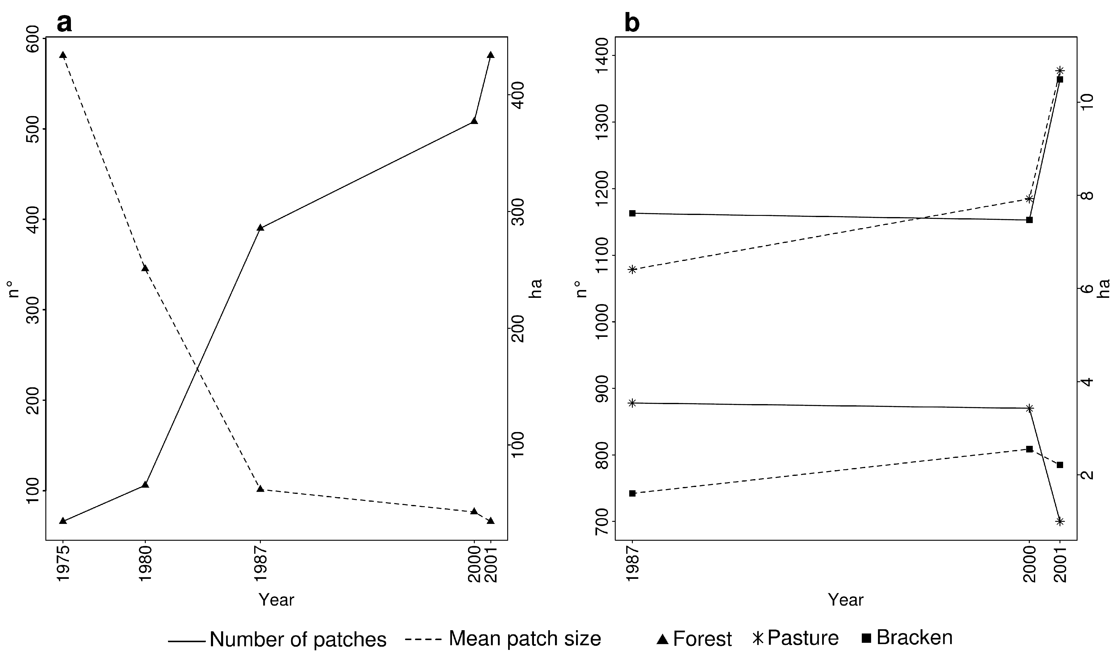
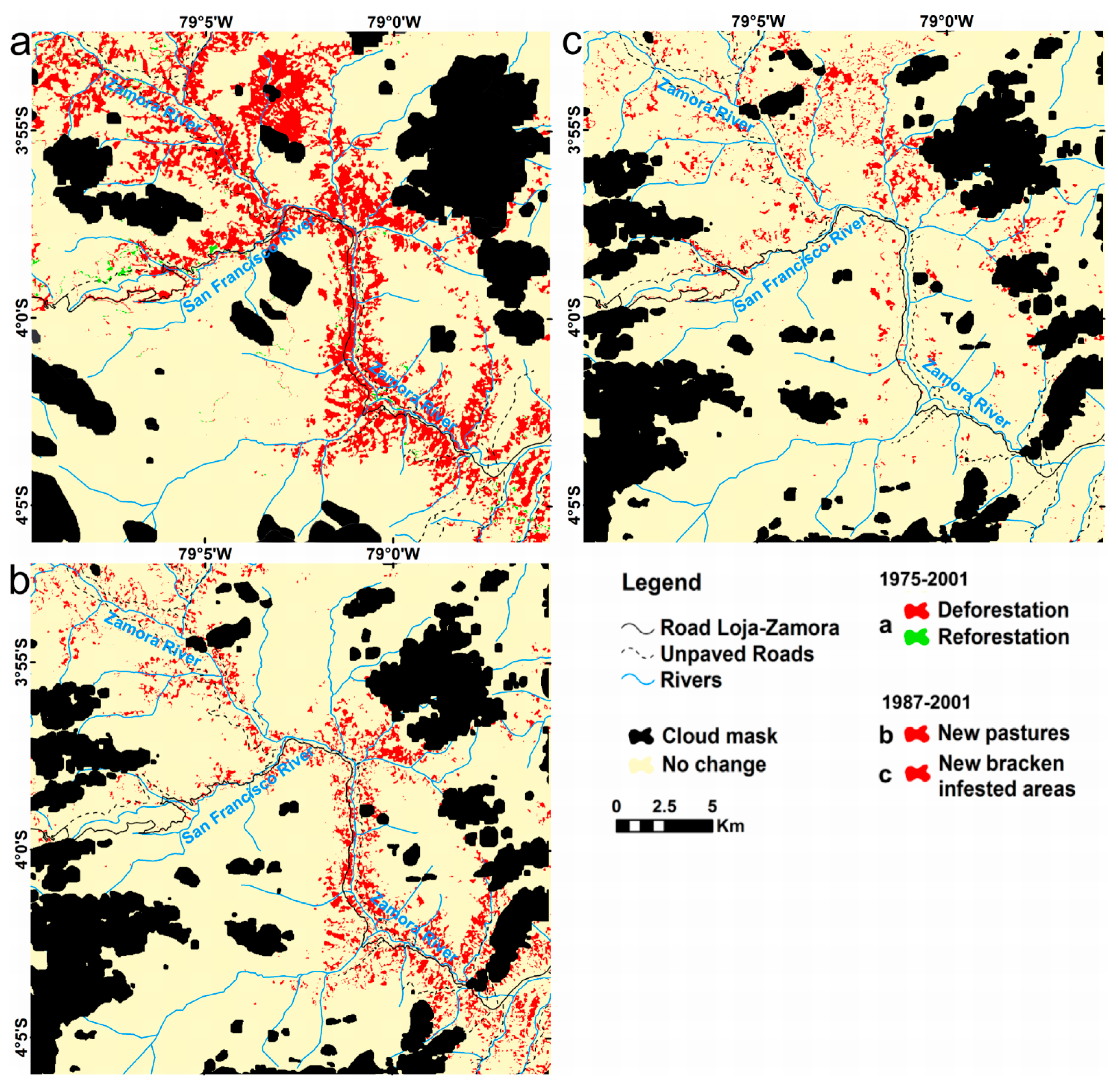
4.3. Land Cover Change and Habitat Fragmentation

In 1975 ~28,500 ha (88.5% of the study area) were covered by forest. By 2001, ~8500 ha (~20% of the study area) were deforested and mainly converted into pastures or invaded by bracken fern (Table 6; Figure 7). The annual deforestation rate between 1980 and 2000 was 1%, which is slightly lower compared to the rate of 1.3% calculated by the Food and Agriculture Organization (FAO) [90] for the whole of Ecuador in the same period.

Table 6. Annual deforestation rates and area of the main land cover classes in the studied periods/years.

**Table 6.** Annual deforestation rates and area of the main land cover classes in the studied periods/years.
	1975		1980		1987		2000		2001
Annual Deforestation Rate (%)		1.5		1.4		0.8		7.5
	Ha	%	Ha	%	Ha	%	Ha	%	Ha	%
Forest	28,617	88.5	26,586	82.2	24,084	74.4	21,611	66.8	19,980	61.8
Pasture	3110	9.6	4873	15.1	5627	17.4	6895	21.3	7473	23.1
Bracken	3110	9.6	4873	15.1	1865	5.8	2943	9.1	3017	9.3
Burnt	626	2	894	2.8	2	0.0	74	0.2	892	2.8
Non-vegetated	626	2	894	2.8	754	2.3	809	2.5	970	3.0

In the first two periods (1975–1980 and 1980–1987) the annual deforestation rate was ~1.5%. In the third period (1987–2000) it slowed down to approximately half (0.8%), while in the fourth period (2000–2001) an extremely high deforestation rate of 7.5% was observed. A big fire event (see Figure 7e, upper middle of the scene), which accounted for 3.5% of the deforestation rate in that year, contributed to this high rate.

From 1987 to 2001 the massive conversion of forest into pastures (1846 ha) and bracken-infested areas (1152 ha), the higher increase of bracken-infested areas (~62%) in comparison to pastures (~33%), and the fact that a high percentage of pastures (13% from 1987 to 2000 and 5.6% from 2000 to 2001) was invaded by bracken are proofs of the necessity of more sustainable land use practices without the use of fire. On the other hand, an unexpected and positive result is the considerable amount of bracken-infested areas that were converted to pastures (29.1% from 1987 to 2000 and 26.4% from 2000 to 2001) or reforested (18% from 1987 to 2000 and 8.9% from 2000 to 2001; Table 7). This practice of converting bracken-infested areas into pastures or reforestation areas, if strengthened, could be a measure to alleviate, at least in the short to medium term, the pressure on the natural forest. As described by Knoke et al. [48], reforestation of bracken-infested areas could reduce deforestation by up to 45% and, at the same time, may increase farmers’ profits by up to 65%.

From 1975 to 2001, an accelerated forest fragmentation tendency was observed. Forest patches increased from 66 to 581 and the mean forest patch size decreased from 433 to 34 ha (Figure 8a). Forest patches are characterized by dry fire-prone edges that neighbor frequently burned pastures [91] or dry bracken fern-dominated vegetation [39]. Moreover, they are often degraded by logging, which increases the process of desiccation and fuel loading [92]. Hence, as fire is frequently used in our study area, fragmentation may further increase the ecosystem vulnerability to fires [93] by positive feedback loops, leading to further forest degradation and loss [18,92,94].

Table 7. Transition matrices of land cover change in the periods 1975–1980, 1980–1987, 1987–2000, and 2000–2001.

**Table 7.** Transition matrices of land cover change in the periods 1975–1980, 1980–1987, 1987–2000, and 2000–2001.
	1980	Forest	Pasture/Bracken	Non-Vegetated
1975	Forest	94	4.8	1.2
	Pasture/Bracken	8.2	87.2	4.6
	Non-vegetated	12.4	37.7	49.9
	1987	Forest	Pasture	Bracken	Burnt	Non-Vegetated
1980	Forest	90.2	5.8	3.1	0	0.9
	Pasture/Bracken	13.3	71.1	12.5	0	3.1
	Non-vegetated	13.8	23.6	20.3	0	42.3
	2000	Forest	Pasture	Bracken	Burnt	Non-Vegetated
1987	Forest	86.3	8.1	4.7	0.3	0.6
	Pasture	8.8	74.8	13	0	3.4
	Bracken	18	29.1	50.7	0.3	1.9
	Burnt	87	0	13	0	0
	Non-vegetated	17.6	16.9	13.8	0	51.7
	2001	Forest	Pasture	Bracken	Burnt	Non-Vegetated
2000	Forest	89.6	2.9	3.5	3.7	0.3
	Pasture	7.1	85.2	5.6	0	2.1
	Bracken	8.9	26.4	61	1.7	2
	Burnt	1.1	3.1	34.6	61.1	0.1
	Non-vegetated	3.8	8.5	2.9	0	84.8

From 1987 to 2001, pasture patches decreased from 878 to 700, while the mean size increased from 6.4 to 10.7 ha (Figure 8b). This trend shows a steady expansion of pasture lands around the existing pasture areas, particularly noticeable between 2000 and 2001.

Figure 8. Number of patches and mean patch size of (a) forest and (b) pasture and bracken.

Between 1987 and 2000, the number of bracken patches remained almost constant but the mean patch size increased from ~1.6 to ~2.6 ha (Figure 8b). Burning for pasture maintenance or expansion affected adjacent dry bracken-infested areas and the vulnerable borders of disturbed forest. Burnt forest edges were invaded by bracken and hence bracken patches expanded. This mechanism confirms the observations on forest-to-bracken cover change patterns observed in the field [37].

Between 2000 and 2001, the bracken spatial pattern was considerably affected by a big fire event. The number of bracken patches rapidly increased from 1153 to 1364 and the mean patch size decreased to 2.2 ha (Figure 8b). As shown in Figure 7c (in the upper middle sector), bracken started to rapidly spread in a patchy way after the fire event. However, at the time of the image acquisition in 2001 it had not yet colonized the complete burned area.

The use of two different spatial resolutions in the change detection analysis may result in a bias, because small-scale changes are only detected in the higher resolution data. By quantifying this deviation, we found a potential average bias of ~9% for the deforestation change trajectories between the Landsat MSS scenes (60 m of spatial resolution) and the Landsat TM and ETM+ scenes (30 m of spatial resolution), because only ~6% to ~12% of the deforested area was not detected if the 30 m spatial resolution data of the periods 1987–2000 and 2000–2001 was resampled to 60 m resolution (Figure 9). This implies that the use of multiresolution maps in this study only introduces small errors since ~90% of the deforested patches were detected when the resolution was coarsened to 60 m. Even when the deforestation maps were further coarsened to 240 m, ~50% of deforested patches were still detected.

Figure 9. Detected deforested area (relative to 60 m resolution) in the periods 1975–1980, 1980–1987, 1987–2000, and 2000–2001 at different spatial resolutions.

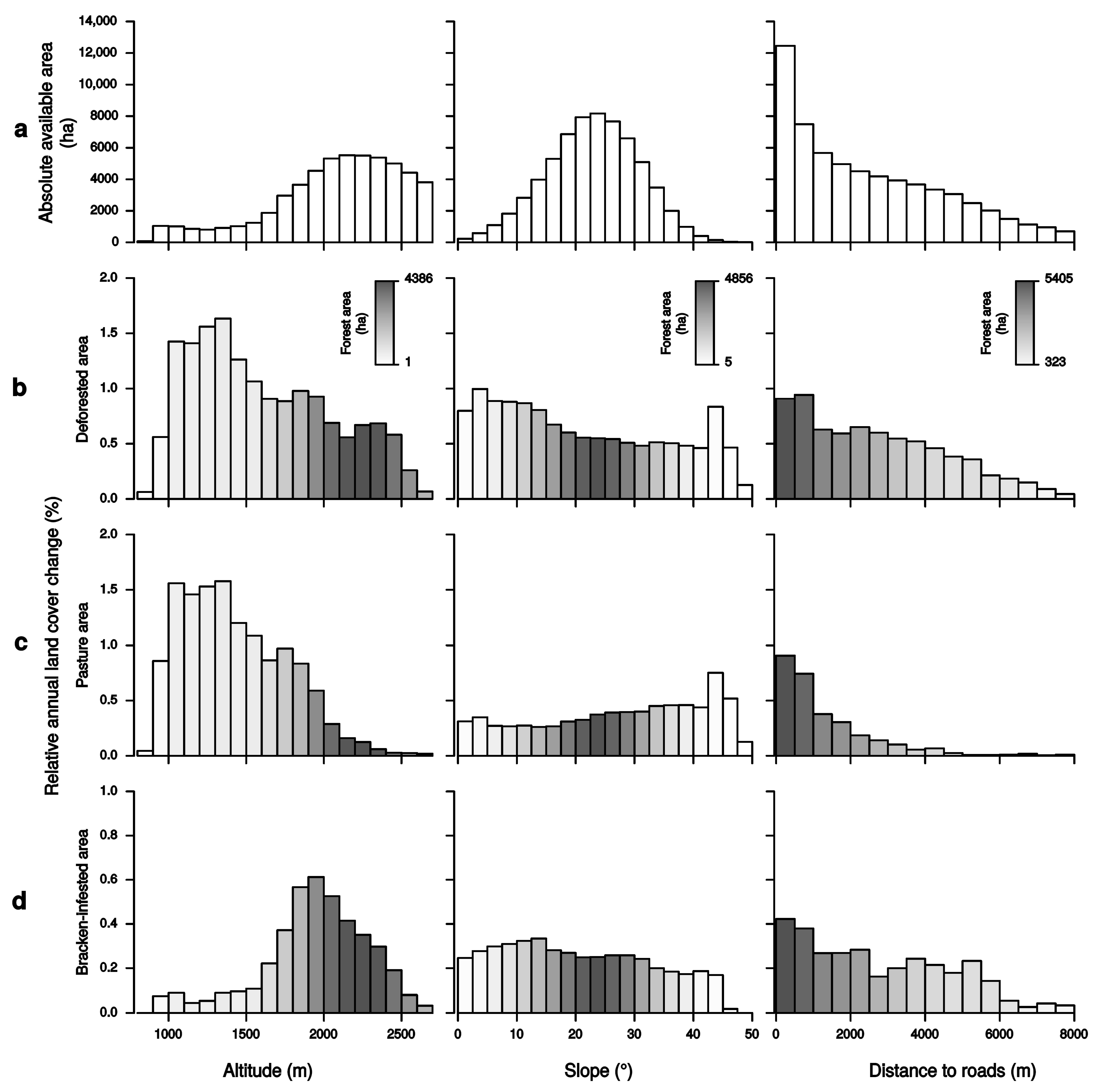
4.4. Land Cover Change in Relation to Distance from Roads, Altitude, and Slope

As in other studies in montane forest areas [95] and in the Amazon lowlands [88,96,97,98,99], we identified roads as the most significant attractor of landscape change and proximate driver of deforestation (Figure 10a and Figure 11).

Between 1987 and 2001, new pastures were mostly created along the road Loja-Zamora, from Zamora city upstream until the confluence with the San Francisco River (Figure 10b) at altitudes between 1000 to 1500 m a.s.l. (Figure 11c). On the other hand, bracken-infested areas occurred mostly in the Upper Zamora River Basin and not always close to roads (Figure 10c). New bracken-infested areas mainly formed at higher altitudes than pastures (between 1800 and 2100 m a.s.l.; Figure 11d), possibly due to the higher competitiveness of bracken under colder and moister conditions [100]. Moreover, this altitudinal range coincides with the altitudinal range where both bracken fern species coexist (1500 and 2400 m a.s.l.) [101].

Figure 10. (a) Change in forest cover between 1975 and 2001; and (b) new pasture and (c) bracken-infested areas in the period 1987–2001.

In a recent study, Laurance et al. [102] pinpointed the Andes of Ecuador as a “conflict area” for road construction, given its high agricultural economic potential, high biodiversity, and provision of valuable ecosystem services. Considering the history of land cover change in the southeastern Ecuadorian Andes, with roads as major attractors of deforestation, any future expansion of road infrastructure as foreseen by the National Strategic Mobility and Transport Plan (PEM) in Ecuador should be addressed with extreme care to avoid serious environmental impacts with irreversible consequences.

We would have expected to find more new bracken-infested areas on steeper slopes where pastures are less wanted [103]. However, new bracken-infested areas were found in flatter slopes compared to pastures (Figure 11c,d). The reason why pastures were found on steeper slopes can be explained by the expansion of old pastures into steeper neighboring lands, and by the depletion of flat areas near the roads. Bracken fern expands rapidly where burnt areas or poorly maintained pastures exist and where it has competitive advantages. Its lower invasion rate in steeper areas corresponds to the relatively open canopy of bracken’s horizontal-oriented fronds, which facilitate the penetration of wind-dispersed seeds from competitor species and light [44,45,101].

Figure 11. Bar plots of absolute available area (first row, a) in relation to altitude (left column), slope (center), and distance to roads (right). The other figures depict the relative annual land cover change between 1987 and 2001 regarding deforested areas (second row, b), pasture lands (third row, c), and bracken-infested areas (fourth row, d) with respect to the same attractors of land cover change. The grey tones of the bars indicate the total available area covered by forest (in hectares).

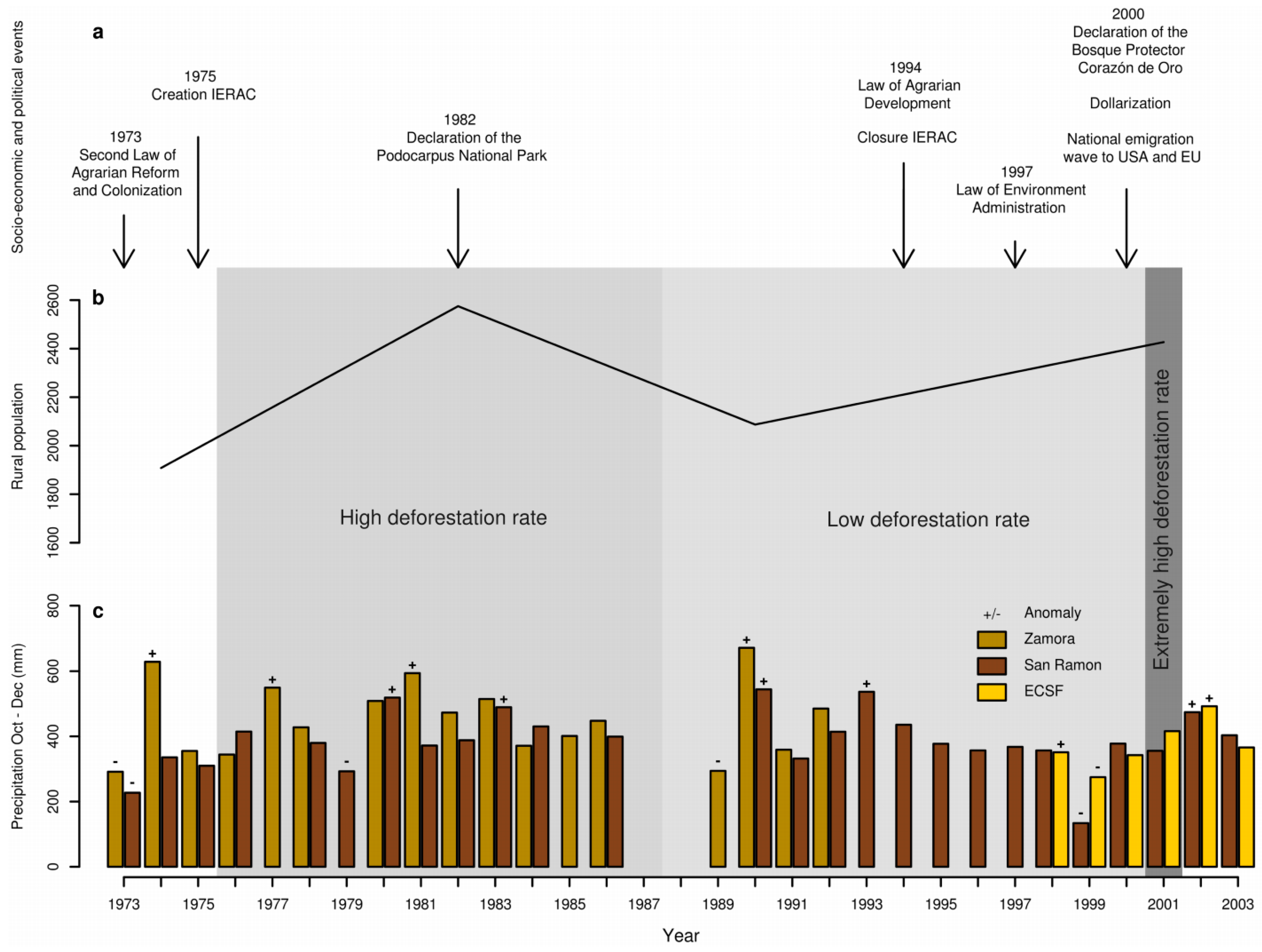
4.5. Potential Deforestation Drivers

The main potential drivers supposed to affect the different deforestation rates found in the studied periods are summarized in Figure 12. The link between potential drivers, actors, and deforestation will be discussed in the following sections.

Figure 12. Potential drivers (a–c) responsible for the changes in the deforestation level (gray tones in the background) derived from the remote sensing analysis in the study area. (a) Sociopolitical and economic events; (b) absolute rural population number for the three parishes acquired from the Ecuadorian Instituto Nacional de Estadística y Censos (INEC); and (c) precipitation amount in the driest months (October to December) and anomalous years in the period between 1966 and 2011, obtained and compiled from the data collected by three meteorological stations within the area of investigation. The ECSF station, located at 1960 m a.s.l., collected data since 1998 [104]; the San Ramón station (1820 m a.s.l.) from the Empresa Eléctrica Regional del Sur S.A. (EERSSA) provided data from 1964 until 2008; and the Zamora station (970 m a.s.l.) from the Instituto Nacional de Meteorología e Hidrología (INAMHI) collected data from 1964 until 1993. The anomalous years were calculated as ≥ +1 or ≤ −1 standard deviation (σ) based on all data collected.

4.5.1. Precipitation during the Dry Season

The Mestizo and Saraguro’s land use system is highly dependent on weather. During the dry spells of the pre-humid Andes, farmers are used to burning land. Particularly, fires during drier periods favor fire dispersion and hence deforestation [93,105,106]. Therefore, we expected higher deforestation particularly if precipitation amounts during the dry season exhibit a clear negative anomaly.

Results, however, showed no relationship between the frequency of negative precipitation (or drought) anomalies (rainfall less than average rain −1 standard deviation) during the dry seasons and higher deforestation rates in the studied time frames (Figure 12c): The period 1975–1987 was characterized by a high deforestation rate of ~1.5%, but only one dry season presented a negative precipitation anomaly; for 1987–2000, with a deforestation rate of ~0.8%, we identified two negative precipitation anomalies. Finally, the extremely high deforestation rate observed in the period 2000–2001 does not coincide with any drought anomaly.

4.5.2. Rural Population Dynamics

From 1974 until 2001, the rural population in the study area increased from 1908 to 2427 inhabitants (Figure 12b). Annual growth rates varied in the observation periods: ~4.5% between 1974 and 1982, a decrease of −2.5% between 1982 and 1990, and a very small increase of ~1.5% between 1990 and 2001.

Consistently with many other studies in other regions [20,107,108,109], we found a correspondence between population increment and the decrease of forest coverage in the first observation period (1975–1980). Likewise, the lower rate of deforestation between 1987 and 2000 is probably a result of a decrease in rural population between 1982 and 1990 as well. However, the increase in population between 1990 and 2001 does not have a repercussion in forest loss dynamics. The latter suggests that other drivers or a combination of these (including population change) may have a stronger relevance in explaining forest cover change, as will be discussed in the next section.

4.5.3. Socioeconomic and Political Factors

Despite the national economic growth in Ecuador at the end of the 1960s and 1970s based on the discovery of oil in the north east and its export [110], a severe drought in Loja province in 1968 and the finalization of the Loja-Zamora road in 1962 resulted in the migration of thousands of smallholders to other regions of the country, including the study area [111].

Moreover, with the Agrarian Reform and Colonization Laws of 1964 and 1973, land clearing became the main condition for access to land titles, [9] and these to credits [112]. Land titles were issued at the regional office of the National Institute of Agrarian Reform and Colonization (IERAC) in Zamora city, which was opened in 1975. In accordance with the findings of Southgate et al. [9], Wunder [113], and Alvarez and Naughton-Treves [96] elsewhere, the high deforestation rate in the period 1975–1987 can be explained by the high number of newcomers conducting subsistence agriculture, their need for land, and the policies facilitating land titles and credits in non-forested areas (Figure 12a).

During the 1980s and 1990s, the Ecuadorian economy faced severe budget crises, high fluctuations of the export prices of oil, currency devaluations, earthquakes that heavily affected oil production, and a frontier war with Peru in 1995. The period 1997–1998 brought a very destructive El Niño event and the Asian economic crisis. In this period the government reduced credits offered to the farmers and the Agrarian Development Law in 1994 eliminated the condition of forest clearing for adjudications [43]. The IERAC office was closed and land titling processes were suspended from 1996 to 2002.

Parallel to these events, since the mid-1990s, as the Ministry of the Environment was created and the Law of Environment Administration was issued, the influence of environmental policy regarding protected areas became an issue in the country. In the study area, the declaration of the Podocarpus National Park (in 1982) allocated land to conservation purposes, despite lack of information among the local population. Formally, this declaration settled legal barriers to the conversion of forests to agricultural land and to the acquisition of property titles.

Between the 1970s and the end of the 1990s, there arose a rush for romerillo timber (Podocarpus oleifolius and Prumnopitys montana) in the study area, which brought a noticeably large gross income that was in part redeemed by the high costs of extraction [113]. Settlers were involved in the selective extraction of the few wild growing high value timber species and thus had less interest and time to invest in clearing forest for new pastureland. All these facts could explain the lower deforestation rate in the period 1987–2000 (Figure 12a).

By the end of the 1990s, romerillo timber became scarce in the study area. Due to the extractive activity, the forest had already suffered disturbance through microclimatic alterations and an increase in the understory litter, resulting in a higher susceptibility to fire [114]. Moreover, since 1997 the authorities had begun to confiscate timber transported without permission [37] and extensive cattle farming turned into the unique relevant production activity.

In the same period, Ecuador’s economy was in a tailspin of hyperinflation, which provoked the default of the foreign debt, the collapse of the Ecuadorian bank sector, high unemployment rates, and finally, the dollarization of the national currency at the beginning of 2000 [115]. The crises led to an extremely high migration to the USA and the EU, especially during the end of the 1990s [116,117]. Wunder and Sunderlin [118] expected lower deforestation in the period after the dollarization due to the loss of competitiveness, which harms the land-using sectors. Messina and Cochrane [18] relate the dollarization with land abandonment, forest transition, and a possible migration to other forested areas in the north Ecuadorian lowlands.

As in other regions of the country, Gerique [37] reports that several settlers migrated to Spain due to the economic crisis. Nonetheless, as previously found by Jokisch [119], Carr [120], Gray [121], and Gray and Bilsborrow [122], our results suggest that emigration did not lead to agricultural abandonment. The dollarization could have led people directly affected by the crisis and with more possibilities to move outside the country. However, poor people in rural areas, which did not have US money at their disposal, probably opted to increase subsistence agriculture or to expand their property as a security measure. In other tropical countries like Cameroon and Indonesia, it was found that economic crises motivated farmers to clear land [123] to, among other reasons, increase income security [124], particularly due to the rising prices of milk.

Furthermore, the profound mistrust of the banking sector after the crisis and the credit and financing difficulties in the agrarian sector could have provoked a relevant part of the remittances sent by the migrants, which were the second most important source of income for the country in 2000 [125], being invested in a way that resulted in the expansion of pastures. Cattle ranching is preferred to the production of crops because of many reasons: (i) the prices of milk and meat in regional markets are more stable than those of other products; (ii) the income is higher; (iii) it is less risky; and (iv) it awards a prestigious social status because it enables an accumulation of capital in regions with unsure loan and pension systems [37,62,126,127]. Stoorvogel et al. [128] mention that in this period the production of milk was preferred to other activities because it did not require expensive external inputs. Guerrero Cazar and Ospina Peralta [125] show that in 1999 even the farm gate prices had grown by 30.8% for cattle and 35.9% for milk. However, as in other areas of Ecuador [119], remittances were probably not dedicated to technological improvements of agricultural production, nor to diversification, but to the expansion of arable land.

The extremely high deforestation rate between 2000 and 2001 is then most probably an indirect effect of the wood scarcity and strengthened controls on wood extraction, and in particular a consequence of the economic crisis in the livelihood of the local population (Figure 12a). There were only two options for lumberjacks in particular and for local livelihoods in general, to abandon the area or to invest in cattle ranching as a mean of subsistence. In addition, even if it has been proven that protected areas [88], particularly in the Amazon, can act as effective barriers against forest fires and deforestation [129,130], the big fire (see Figure 7e) revealed by the satellite image classification within the perimeter of the Corazón de Oro Protected Forest (created in June 2000) shows that bad fire management and weak governance, especially during times of economic crisis, are important issues to be addressed with regard to forest protection.

5. Conclusions

The described semi-automated pre-processing framework for Landsat satellite data provides a solid basis for land cover change analysis in the tropical Andes of southeastern Ecuador. Although remote sensing applications in this area are challenging because the complex topography distorts the satellite signal and the high cloud frequency complicates the acquisition of images, we achieved good results in the correction of five Landsat scenes from 1975 to 2001, an essential step towards accurately classifying the land cover. To our knowledge, this is the longest period of satellite-based land cover change research in the region and it is the first time that an analysis of the fire–bracken–pasture dynamics has been included.

Between 1975 and 2001, in the Upper Zamora and San Francisco Valleys, strong forest loss and habitat fragmentation originated in the need for pasture expansion. However, non-sustainable fire practices accounted for almost one third of forest loss and degradation of usable land resources. The issue of burning more land than required supported the infestation of the land by bracken, whose spatial expansion was two times faster than pastureland between 1987 and 2001. The increase in forest patches and the decrease in their mean size, which made the remaining forest more vulnerable to fire, led to the observed rapid expansion of bracken fern surface. To our surprise, a considerable percentage of bracken-infested areas was also converted to pastureland, a practice that could alleviate pressure on forests if further supported by incentives.

The most important spatial element conditioning deforestation was the proximity to roads, given that pastures are easily reachable. Pasture expansion resulted in the use of neighboring areas at higher slopes. Bracken colonized all unused burnt areas and poorly managed pastures, with a higher incidence on flatter slopes. A higher increase in new pasture areas was found at lower elevations, while the altitudinal range where most of the new bracken-infested areas appeared coincided with the altitudes where both bracken fern species coexist.

Land cover change detection revealed that the deforestation rate in the study area was highly variable between 1975 and 2001. Precipitation during the dry season was not a relevant driver in any of the studied periods. The high deforestation from 1975 to 1987 is explained by the recently arrived settlers, who were motivated by land use policies favoring land titles and credit. The deforestation slowdown between 1987 and 2000 seems to be related to a decrease in the rural population, the cessation of the aforementioned land use policies, and more selective timber extraction activity. The creation of the Podocarpus National Park and the new environmental laws apparently helped forest protection as well. The extremely high deforestation between 2000 and 2001 is partially explained by wood scarcity and strengthening of controls over wood since the end of the 1990s, which made cattle ranching the only profitable productive activity. Still, we strongly believe that the economic crisis in Ecuador, which led to the dollarization in 2000 and to a national emigration wave to USA and EU, motivated farmers to expand their properties and clear more forest as a security measure, while emigrants contributed to this expansion through remittances. This is a subject that would merit more attention in future works.

Acknowledgments

We thank the foundation Naturaleza y Cultura Internacional (NCI) Loja for logistic support and the Ministry of the Environment of Ecuador (MAE) for the research permission (024-IC-AGUA-DPL-MA). We are grateful to Thorsten Peters for ECSF climate data provision (doi:10.5678/lcrs/for816.dat.497); to Dirk Hattermann, Alexander Groos, Hanna Meyer, Bianca Regeling, Julian Öser, and Daniel Baron for help in data processing; to André Obregón, Rütger Rollenbeck, Mariana Alvarado Chávez, Maik Dobbermann, M. Ximena Fernández Fontenoy, and in particular to Sandro Makowski Giannoni for their valuable advice and for helpful comments on the paper. We finally thank the editors and the three anonymous reviewers for their valuable comments and corrections.

Author Contributions

Giulia F. Curatola Fernández, Wolfgang A. Obermeier, Lukas W. Lehnert, and Jörg Bendix conceived and designed the experiments; Giulia F. Curatola Fernández, Wolfgang A. Obermeier, and Lukas W. Lehnert performed the experiments; Giulia F. Curatola Fernández, Wolfgang A. Obermeier, Andrés Gerique, María Fernanda López Sandoval, and Lukas W. Lehnert analyzed the data; Lukas W. Lehnert and Boris Thies contributed analysis tools; and Giulia F. Curatola Fernández wrote the paper with contributions from all coauthors.

Conflicts of Interest

The authors declare no conflict of interest.

References

Foley, J.A.; DeFries, R.; Asner, G.P.; Barford, C.; Bonan, G.; Carpenter, S.R.; Chapin, F.S.; Coe, M.T.; Daily, G.C.; Gibbs, H.K.; et al. Global consequences of land use. Science 2005, 309, 570–574. [Google Scholar] [CrossRef] [PubMed]
Myers, N.; Mittermeier, R.A.; Mittermeier, C.G.; da Fonesca, G.A.B.; Kent, J. Biodiversity hotspots for conservation priorities. Nature 2000, 403, 853–858. [Google Scholar] [CrossRef] [PubMed]
Asner, G.P.; Loarie, S.R.; Heyder, U. Combined effects of climate and land-use change on the future of humid tropical forests. Conserv. Lett. 2010, 3, 395–403. [Google Scholar] [CrossRef]
Hansen, M.C.; Potapov, P.V; Moore, R.; Hancher, M.; Turubanova, S.A.; Tyukavina, A.; Thau, D.; Stehman, S.V; Goetz, S.J.; Loveland, T.R.; et al. High-resolution global maps of 21st-century forest cover change. Science 2013, 342, 850–853. [Google Scholar] [CrossRef] [PubMed]
Sierra, R.; Stallings, J. The dynamics and social organization of tropical deforestation in northwest Ecuador, 1983–1995. Hum. Ecol. 1998, 26, 135–161. [Google Scholar] [CrossRef]
Grau, H.R.; Aide, M. Globalization and land-use transitions in Latin America. Ecol. Soc. 2008, 13, 16. [Google Scholar]
Lambin, E.F.; Meyfroidt, P. Land use transitions: Socio-ecological feedback versus socio-economic change. Land Use Policy 2010, 27, 108–118. [Google Scholar] [CrossRef]
Sierra, R. The role of domestic timber markets in tropical deforestation and forest degradation in Ecuador: Implications for conservation planning and policy. Ecol. Econ. 2001, 36, 327–340. [Google Scholar] [CrossRef]
Southgate, D.; Sierra, R.; Brown, L. The causes of tropical deforestation in Ecuador: A statistical analysis. World Develp. 1991, 19, 1145–1151. [Google Scholar] [CrossRef]
Pichón, F. Settler households and land-use patterns in the Amazon frontier: Farm-level evidence from Ecuador. World Develop. 1997, 25, 67–91. [Google Scholar] [CrossRef]
Sierra, R. Dynamics and patterns of deforestation in the western Amazon: The Napo deforestation front, 1986–1996. Appl. Geogr. 2000, 20, 1–16. [Google Scholar] [CrossRef]
Messina, J.; Walsh, S. 2.5 D Morphogenesis: Modeling land use and land cover dynamics in the Ecuadorian Amazon. Plant Ecol. 2001, 156, 75–88. [Google Scholar] [CrossRef]
Pan, W.K.Y.; Walsh, S.J.; Bilsborrow, R.E.; Frizzelle, B.G.; Erlien, C.M.; Baquero, F. Farm-level models of spatial patterns of land use and land cover dynamics in the Ecuadorian Amazon. Agr. Ecosyst. Environ. 2004, 101, 117–134. [Google Scholar] [CrossRef]
Viña, A.; Echavarria, F.R.; Rundquist, D.C. Satellite change detection analysis of deforestation rates and patterns along the Colombia-Ecuador border. Ambio 2004, 33, 118–125. [Google Scholar] [PubMed]
Pan, W.K.Y.; Bilsborrow, R.E. The use of a multilevel statistical model to analyze factors influencing land use: A study of the Ecuadorian Amazon. Global Planet Change 2005, 47, 232–252. [Google Scholar] [CrossRef]
Mena, C.F.; Bilsborrow, R.E.; McClain, M.E. Socioeconomic drivers of deforestation in the Northern Ecuadorian Amazon. Environ. Manag. 2006, 37, 802–815. [Google Scholar] [CrossRef]
Messina, J.P.; Walsh, S.J.; Mena, C.F.; Delamater, P.L. Land tenure and deforestation patterns in the Ecuadorian Amazon: Conflicts in land conservation in frontier settings. Appl. Geogr. 2006, 26, 113–128. [Google Scholar] [CrossRef]
Messina, J.P.; Cochrane, M.A. The forests are bleeding: How land use change is creating a new fire regime in the Ecuadorian Amazon. J. Lat. Am. Geogr. 2007, 6, 85–100. [Google Scholar] [CrossRef]
López, S.; Sierra, R. Agricultural change in the Pastaza River Basin: A spatially explicit model of native Amazonian cultivation. Appl. Geogr. 2010, 30, 355–369. [Google Scholar] [CrossRef]
Mena, C.F.; Walsh, S.J.; Frizzelle, B.G.; Xiaozheng, Y.; Malanson, G.P. Land use change on household farms in the Ecuadorian Amazon: Design and implementation of an agent-based model. Appl. Geogr. 2011, 31, 210–222. [Google Scholar] [CrossRef] [PubMed]
López, S.; Beard, R.; Sierra, R. Landscape change in western Amazonia. Geogr. Rev. 2013, 103, 37–58. [Google Scholar] [CrossRef]
Holland, M.B.; de Koning, F.; Morales, M.; Naughton-Treves, L.; Robinson, B.E.; Suárez, L. Complex tenure and deforestation: Implications for conservation incentives in the Ecuadorian Amazon. World Develp. 2014, 55, 21–36. [Google Scholar] [CrossRef]
Sierra, R. Traditional resource-use systems and tropical deforestation in a multi-ethnic region in North-West Ecuador. Environ. Conserv. 1999, 26, 136–145. [Google Scholar] [CrossRef]
López, S.; Sierra, R.; Tirado, M. Tropical deforestation in the Ecuadorian Chocó: Logging practices and socio-spatial relationships. Geogr. Bull. 2010, 51, 3–22. [Google Scholar]
Colby, J.D.; Keating, P.L. Land cover classification using Landsat TM imagery in the tropical highlands: The influence of anisotropic reflectance. Int. J. Remote Sens. 1998, 19, 1479–1500. [Google Scholar] [CrossRef]
Conese, C.; Maselli, F. Use of multitemporal information to improve classification performance of TM scenes in complex terrain. ISPRS J. Photogramm. Remote Sens. 1991, 46, 187–197. [Google Scholar] [CrossRef]
Martinuzzi, S.; Gould, W.A.; Ramos González, O.M. Creating Cloud-Free Landsat ETM+ Data Sets in Tropical Landscapes: Cloud and Cloud-Shadow Removal; General Technical Report IITF-GTR-32; USDA: Washington, DC, USA, February 2007. [Google Scholar]
Elmahboub, W.; Scarpace, F.; Smith, B. A highly accurate classification of TM data through correction of atmospheric effects. Remote Sens. 2009, 1, 278–299. [Google Scholar] [CrossRef]
Richter, R.; Kellenberger, T.; Kaufmann, H. Comparison of topographic correction methods. Remote Sens. 2009, 1, 184–196. [Google Scholar] [CrossRef] [Green Version]
Ediriweera, S.; Pathirana, S.; Danaher, T.; Nichols, D.; Moffiet, T. Evaluation of different topographic corrections for Landsat TM data by prediction of foliage projective cover (FPC) in topographically complex landscapes. Remote Sens. 2013, 5, 6767–6789. [Google Scholar] [CrossRef]
Vanonckelen, S.; Lhermitte, S.; van Rompaey, A. The effect of atmospheric and topographic correction methods on land cover classification accuracy. Int. J. Appl. Earth Obs. Geoinf. 2013, 24, 9–21. [Google Scholar] [CrossRef]
Vanonckelen, S.; Lhermitte, S.; Balthazar, V.; Van Rompaey, A. Performance of atmospheric and topographic correction methods on Landsat imagery in mountain areas. Int. J. Remote Sens. 2014, 35, 4952–4972. [Google Scholar] [CrossRef]
Jokisch, B.D.; Lair, B.M. One last stand? Forests and change on Ecuador’s eastern Cordillera. Geogr. Rev. 2002, 92, 235–256. [Google Scholar] [CrossRef]
Pohle, P.; Gerique, A. Traditional ecological knowledge and biodiversity management in the Andes of southern Ecuador. Geogr. Helv. 2006, 4, 275–285. [Google Scholar] [CrossRef]
Göttlicher, D.; Obregón, A.; Homeier, J.; Rollenbeck, R.; Nauss, T.; Bendix, J. Land cover classification in the Andes of southern Ecuador using Landsat ETM+ data as a basis for SVAT modelling. Int. J. Remote Sens. 2009, 30, 1867–1886. [Google Scholar] [CrossRef]
Pohle, P.; Gerique, A.; Park, M.; López Sandoval, M.F. Human ecological dimensions in sustainable utilization and conservation of tropical mountain rain forests under global change in southern Ecuador. In Tropical Rainforests and Agroforests under Climate Change: Ecological and Socio-econimic Valuations; Tscharntke, T., Leuschner, C., Veldkamp, E., Faust, H., Guhardja, E., Bindin, A., Eds.; Springer: Berlin/Heidelberg, Germany, 2010; pp. 477–509. [Google Scholar]
Gerique, A. Biodiversity as a Resource: Plant Use and Land Use Among the Shuar, Saraguros, and Mestizos in Tropical Rainforest Areas of Southern Ecuador. Ph.D. Thesis, University of Erlangen-Nürnberg, Erlangen, Germany, September 2011. [Google Scholar]
Bendix, J.; Beck, E.; Bräuning, A.; Makeschin, F.; Mosandl, R.; Scheu, S.; Wilcke, W. Ecosystem Services, Biodiversity, and Environmental Change in a Tropical Mountain Ecosystem of South. Ecuador; Springer: Berlin-Heidelberg, Germany, 2013. [Google Scholar]
Curatola Fernández, G.F.; Silva, B.; Gawlik, J.; Thies, B.; Bendix, J. Bracken fern frond status classification in the Andes of southern Ecuador: Combining multispectral satellite data and field spectroscopy. Int. J. Remote Sens. 2013, 34, 7020–7037. [Google Scholar] [CrossRef]
Beck, E.; Bendix, J.; Kottke, I.; Makeschin, F.; Mosandl, R. Gradients in a Tropical Mountain Ecosystem of Ecuador; Springer: Berlin/Heidelberg, Germany, 2008. [Google Scholar]
Goerner, A.; Gloaguen, R.; Makeschin, F. Monitoring of the Ecuadorian mountain rainforest with remote sensing. J. Appl. Remote Sens. 2007, 1, 013527. [Google Scholar] [CrossRef]
Thies, B.; Meyer, H.; Nauss, T.; Bendix, J. Projecting land-use and land-cover changes in a tropical mountain forest of Southern Ecuador. J. Land Use Sci. 2012, 9, 1–33. [Google Scholar] [CrossRef]
Pohle, P.; Gerique, A.; López Sandoval, M.F. Current provisioning ecosystem services for the local population: Landscape transformation, land use, and plant use. In Ecosystem Services, Biodiversity, and Environmental Change in a Tropical Mountain Ecosystem of South Ecuador; Bendix, J., Beck, E., Bräuning, A., Makeschin, F., Mosandl, R., Scheu, S., Wilcke, W., Eds.; Springer: Berlin/Heidelberg, Germany, 2013; pp. 219–234. [Google Scholar]
Hartig, K.; Beck, E. The bracken fern (Pteridium arachnoideum (Kaulf.) Maxon) dilemma in the Andes of Southern Ecuador. Ecotropica 2003, 9, 3–13. [Google Scholar]
Beck, E. Forest clearing by slash and burn. In Gradients in a Tropical Mountain Ecosystem of Ecuador; Beck, E., Bendix, J., Kottke, I., Makeschin, F., Mosandl, R., Eds.; Springer: Berlin/Heidelberg, Germany, 2008; pp. 371–374. [Google Scholar]
Potthast, K.; Hamer, U.; Makeschin, F. Impact of litter quality on mineralization processes in managed and abandoned pasture soils in southern Ecuador. Soil Biol. Biochem. 2010, 42, 56–64. [Google Scholar] [CrossRef]
Knoke, T.; Bendix, J.; Pohle, P.; Hamer, U.; Hildebrandt, P.; Roos, K.; Gerique, A.; López Sandoval, M.F.; Breuer, L.; Tischer, A.; et al. Afforestation or intense pasturing improve the ecological and economic value of abandoned tropical farmlands. Nat. Commun. 2014, 5, 1–12. [Google Scholar] [CrossRef]
Knoke, T.; Weber, M.; Barkmann, J.; Pohle, P.; Calvas, B.; Medina, C.; Aguirre, N.; Günter, S.; Stimm, B.; Mosandl, R.; et al. Effectiveness and distributional impacts of payments for reduced carbon emissions from deforestation. Erdkunde 2009, 63, 365–384. [Google Scholar] [CrossRef]
Lu, D.; Batistella, M.; Moran, E. Multitemporal spectral mixture analysis for Amazonian land-cover change detection. Can. J. Remote Sens. 2004, 30, 87–100. [Google Scholar] [CrossRef]
Wondie, M.; Schneider, W.; Melesse, A.M.; Teketay, D. Spatial and temporal land cover changes in the Simen Mountains National Park, a world heritage site in northwestern Ethiopia. Remote Sens. 2011, 3, 752–766. [Google Scholar] [CrossRef]
Souza, C.M., Jr.; Siqueira, J.V.; Sales, M.H.; Fonseca, A.V.; Ribeiro, J.G.; Numata, I.; Cochrane, M.A.; Barber, C.P.; Roberts, D.A.; Barlow, J. Ten-year Landsat classification of deforestation and forest degradation in the Brazilian Amazon. Remote Sens. 2013, 5, 5493–5513. [Google Scholar] [CrossRef]
Tian, Y.; Yin, K.; Lu, D.; Hua, L.; Zhao, Q.; Wen, M. Examining land use and land cover spatiotemporal change and driving forces in Beijing from 1978 to 2010. Remote Sens. 2014, 6, 10593–10611. [Google Scholar] [CrossRef]
Vittek, M.; Brink, A.; Donnay, F.; Simonetti, D.; Desclée, B. Land cover change monitoring using Landsat MSS/TM satellite image data over West Africa between 1975 and 1990. Remote Sens. 2014, 6, 658–676. [Google Scholar] [CrossRef] [Green Version]
Lambin, E.F.; Turner, B.L.; Geist, H.J.; Agbola, S.B.; Angelsen, A.; Bruce, J.W.; Coomes, O.T.; Dirzo, R.; Fischer, G.; Folke, C.; et al. The causes of land-use and land-cover change: Moving beyond the myths. Global Environ. Change 2001, 11, 261–269. [Google Scholar] [CrossRef]
Bürgi, M.; Hersperger, A.M.; Schneeberger, N. Driving forces of landscape change—Current and new directions. Landscape Ecol. 2004, 19, 857–868. [Google Scholar] [CrossRef]
Folke, C.; Hahn, T.; Olsson, P.; Norberg, J. Adaptive governance of social-ecological systems. Annu. Rev. Environ. Resour. 2005, 30, 441–473. [Google Scholar] [CrossRef]
Carmenta, R.; Parry, L.; Blackburn, A.; Vermeylen, S.; Barlow, J. Understanding human-fire interactions in tropical forest regions: A case for interdisciplinary research across the natural and social sciences. Ecol. Soc. 2011, 16, 53. [Google Scholar]
Richter, M.; Diertl, K.-H.; Emck, P.; Peters, T.; Beck, E. Reasons for an outstanding plant diversity in the tropical Andes of southern Ecuador. Landscape Online 2009, 12, 1–35. [Google Scholar]
Bendix, J.; Rollenbeck, R.; Göttlicher, D.; Nauß, T.; Fabian, P. Seasonality and diurnal pattern of very low clouds in a deeply incised valley of the eastern tropical Andes (South Ecuador) as observed by a cost-effective WebCam. Meteorol. Appl. 2008, 291, 281–291. [Google Scholar] [CrossRef]
Homeier, J.; Werner, F.A.; Gradstein, S.R.; Breckle, S.W.; Richter, M. Potential vegetation and floristic composition of Andean forests in South Ecuador, with a focus on the RBSF. In Gradients in a Tropical Mountain Ecosystem of Ecuador; Beck, E., Bendix, J., Kottke, I., Makeschin, F., Mosandl, R., Eds.; Springer: Berlin-Heidelberg, Germany, 2008; pp. 87–100. [Google Scholar]
Ecuador en cifras—Nacionalidades y pueblos (INEC). 2010. Available online: http://www.ecuadorencifras.com/cifras-inec/nacionalidades.html#tpi=493 (accessed on 28 April 2014).
Marquette, C.M. Settler welfare on tropical forest frontiers in Latin America. Popul. Environ. 2006, 27, 397–444. [Google Scholar] [CrossRef]
Roos, K.; Rollenbeck, R.; Peters, T.; Bendix, J.; Beck, E. Growth of tropical bracken (Pteridium arachnoideum): Response to weather variations and burning. Invasive Plant Sci. Manag. 2010, 3, 402–411. [Google Scholar] [CrossRef]
United States Geological Survey (USGS) EarthExplorer. Available online: http://earthexplorer.usgs.gov/ (accessed on 27 February 2015).
Vermote, E.F.; Tanré, D.; Deuzé, J.L.; Herman, M.; Morcrette, J.-J. Second simulation of the satellite signal in the solar spectrum, 6S: An overview. IEEE Trans. Geosci. Remote Sens. 1997, 35, 675–686. [Google Scholar] [CrossRef]
Kalnay, E.; Kanamitsu, M.; Kistler, R.; Collins, W.; Deaven, D.; Gandin, L.; Iredell, M.; Saha, S.; White, G.; Woollen, J.; et al. The NCEP/NCAR 40-year reanalysis project. Bull. Am. Meteorol. Soc. 1996, 77, 437–471. [Google Scholar] [CrossRef]
National Center for Environmental Prediction/National Center of Atmospheric Research (NCEP/NCAR) Reanalysis 1. Available online: http://www.esrl.noaa.gov/psd/data/gridded/data.ncep.reanalysis.html (accessed on 27 February 2015).
Total Ozone Mapping Spectrometer (TOMS) satellite data. Available online: http://disc.sci.gsfc.nasa.gov/acdisc/TOMS (accessed on 27 February 2015).
Teillet, P.M.; Guindon, B.; Goodenough, D.G. On the slope-aspect correction of multispectral scanner data. Can. J. Remote Sens. 1981, 8, 84–106. [Google Scholar] [CrossRef]
Yang, X.; Lo, C.P. Relative radiometric normalization performance for change detection from multi-date satellite images. Photogramm. Eng. Remote Sens. 2000, 8, 967–980. [Google Scholar]
Singh, A. Spectral separability of tropical forest cover classes. Int. J. Remote Sens. 1987, 8, 971–979. [Google Scholar] [CrossRef]
Hong, G. Image Fusion, Image Registration, and Radiometric Normalization for High Resolution Image Processing. Ph.D. Thesis, University of New Brunswick, Fredericton, NB, Canada, April 2007. [Google Scholar]
Elvidge, C.D.; Yuan, D.; Weerackoon, R.D.; Lunetta, R.S. Relative radiometric normalization of Landsat Multispectral Scanner (MSS) data using a automatic scattergram-controlled regression. Photogramm. Eng. Remote Sens. 1995, 61, 1255–1260. [Google Scholar]
Jordan, E.; Ungerechts, L.; Cáceres, B.; Peñafiel, A.; Francou, B. Estimation by photogrammetry of the glacier recession on the Cotopaxi Volcano (Ecuador) between 1956 and 1997/Estimation par photogrammétrie de la récession glaciaire sur le Volcan Cotopaxi (Equateur) entre 1956 et 1997. Hydrol. Sci. J. 2005, 50, 949–961. [Google Scholar] [CrossRef]
Li, C.; Wang, J.; Wang, L.; Hu, L.; Gong, P. Comparison of classification algorithms and training sample sizes in urban land classification with Landsat Thematic Mapper imagery. Remote Sens. 2014, 6, 964–983. [Google Scholar] [CrossRef]
Li, G.; Lu, D.; Moran, E.; Hetrick, S. Land-cover classification in a moist tropical region of Brazil with Landsat Thematic Mapper imagery. Int. J. Remote Sens. 2011, 32, 8207–8230. [Google Scholar] [CrossRef] [PubMed]
Congalton, R.G. A review of assessing the accuracy of classifications of remotely sensed data. Remote Sens. Environ. 1991, 37, 35–46. [Google Scholar] [CrossRef]
Foody, G.M. Status of land cover classification accuracy assessment. Remote Sens. Environ. 2002, 80, 185–201. [Google Scholar] [CrossRef]
Colditz, R.R.; Acosta-Velázquez, J.; Díaz Gallegos, J.R.; Vázquez Lule, A.D.; Rodríguez-Zúñiga, M.T.; Maeda, P.; Cruz López, M.I.; Ressl, R. Potential effects in multi-resolution post-classification change detection. Int. J. Remote Sens. 2012, 33, 6426–6445. [Google Scholar] [CrossRef]
Fahrig, L. Effects of habitat fragmentation on biodiversity. Annu. Rev. Ecol. Evol. 2003, 34, 487–515. [Google Scholar] [CrossRef]
Nagendra, H.; Munroe, D.K.; Southworth, J. From pattern to process: Landscape fragmentation and the analysis of land use/land cover change. Agr. Ecosyst. Environ. 2004, 101, 111–115. [Google Scholar] [CrossRef]
Fischer, J.; Lindenmayer, D.B. Landscape modification and habitat fragmentation: A synthesis. Global Ecol. Biogeogr. 2007, 16, 265–280. [Google Scholar] [CrossRef]
McGarigal, K.; Cushman, S.; Ene, E. FRAGSTATS v4: Spatial pattern analysis program for categorical and continuous maps. Available online: http://www.umass.edu/landeco/research/fragstats/fragstats.html (accessed on 29 March 2014).
Southworth, J.; Munroe, D.; Nagendra, H. Land cover change and landscape fragmentation—Comparing the utility of continuous and discrete analyses for a western Honduras region. Agr. Ecosyst. Environ. 2004, 101, 185–205. [Google Scholar] [CrossRef]
Šímová, P.; Gdulová, K. Landscape indices behavior: A review of scale effects. Appl. Geogr. 2012, 34, 385–394. [Google Scholar] [CrossRef]
Lele, N.; Nagendra, H.; Southworth, J. Accessibility, demography, and protection: Drivers of forest stability and change at multiple scales in the Cauvery Basin, India. Remote Sens. 2010, 2, 306–332. [Google Scholar] [CrossRef]
Newman, M.E.; McLaren, K.P.; Wilson, B.S. Long-term socio-economic and spatial pattern drivers of land cover change in a Caribbean tropical moist forest, the Cockpit Country, Jamaica. Agr. Ecosyst. Environ. 2014, 186, 185–200. [Google Scholar] [CrossRef]
Southworth, J.; Marsik, M.; Qiu, Y.; Perz, S.; Cumming, G.; Stevens, F.; Rocha, K.; Duchelle, A.; Barnes, G. Roads as drivers of change: Trajectories across the tri-national frontier in MAP, the southwestern Amazon. Remote Sens. 2011, 3, 1047–1066. [Google Scholar] [CrossRef]
Lillesand, T.M.; Kiefer, R.W.; Chipman, J.W. Remote Sensing and Image Interpretation, 6th ed.; Wiley: Hoboken, NJ, USA, 2008; pp. 9–12. [Google Scholar]
State of the World’s Forests (FAO), 2003. Available online: http://www.fao.org/docrep/005/y7581e/y7581e00.htm (accessed on 21 March 2014).
Nepstad, D.C.; Veríssimo, A.; Alencar, A.; Nobre, C.; Lima, E.; Lefebvre, P.; Schlesinger, P.; Potter, C.; Moutinho, P.; Mendoza, E.; et al. Large-scale impoverishment of Amazonian forests by logging and fire. Nature 1999, 398, 505–508. [Google Scholar] [CrossRef]
Cochrane, M.A.; Laurance, W.F. Fire as a large-scale edge effect in Amazonian forests. J. Trop. Ecol. 2002, 18, 311–325. [Google Scholar] [CrossRef]
Cochrane, M.A.; Schulze, M.D. Fire as a recurrent event in tropical forests of the eastern Amazon: Effects on forest structure, biomass, and species composition. Biotropica 1999, 31, 2–16. [Google Scholar]
Cochrane, M.A.; Laurance, W.F. Synergisms among fire, land use, and climate change in the Amazon. Ambio 2008, 37, 522–527. [Google Scholar] [CrossRef] [PubMed]
Young, K.R. Roads and the environmental degradation of tropical montane forests. Conserv. Biol. 1994, 8, 972–976. [Google Scholar] [CrossRef]
Alvarez, N.L.; Naughton-Treves, L. Linking national agrarian policy to deforestation in the Peruvian Amazon: A case study of Tambopata, 1986–1997. Ambio 2003, 32, 269–274. [Google Scholar] [PubMed]
Laurance, W.F.; Albernaz, A.K.M.; Fearnside, P.M.; Vasconcelos, H.L.; Ferreira, L.V. Deforestation in Amazonia. Science 2004, 304, 1109–1111. [Google Scholar] [CrossRef] [PubMed]
Sun, J.; Southworth, J. Remote sensing-based fractal analysis and scale dependence associated with forest fragmentation in an Amazon tri‑national frontier. Remote Sens. 2013, 5, 454–472. [Google Scholar] [CrossRef]
Barber, C.P.; Cochrane, M.A.; Souza, C.M., Jr.; Laurance, W.F. Roads, deforestation, and the mitigating effect of protected areas in the Amazon. Biol. Conserv. 2014, 177, 203–209. [Google Scholar] [CrossRef]
Silva, B.; Roos, K.; Voss, I.; König, N.; Rollenbeck, R.; Scheibe, R.; Beck, E.; Bendix, J. Simulating canopy photosynthesis for two competing species of an anthropogenic grassland community in the Andes of southern Ecuador. Ecol. Modell. 2012, 239, 14–26. [Google Scholar] [CrossRef]
Roos, K. Tropical Bracken, a Powerful Invader of Pastures in South Ecuador: Species Composition, Ecology, Control Measures, and Pasture Restoration. Ph.D. Thesis, University of Bayreuth, Bayreuth, Germany, July 2010. [Google Scholar]
Laurance, W.F.; Clements, G.R.; Sloan, S.; O’Connell, C.S.; Mueller, N.D.; Goosem, M.; Venter, O.; Edwards, D.P.; Phalan, B.; Balmford, A.; et al. A global strategy for road building. Nature 2014, 513, 229–234. [Google Scholar] [CrossRef] [PubMed]
Rudel, T.K.; Bates, D.; Machinguiashi, R. A tropical forest transition? Agricultural change, out-migration, and secondary forests in the Ecuadorian Amazon. Ann. Assoc. Am. Geogr. 2002, 92, 87–102. [Google Scholar] [CrossRef]
Rollenbeck, R.; Bendix, J.; Fabian, P.; Boy, J.; Dalitz, H.; Emck, P.; Oesker, M.; Wilcke, W. Comparison of different techniques for the measurement of precipitation in tropical montane rain forest regions. J. Atmos. Ocean. Technol. 2007, 24, 156–168. [Google Scholar] [CrossRef]
Davidson, E.A.; de Araújo, A.C.; Artaxo, P.; Balch, J.K.; Brown, I.F.; Bustamante, M.M.C.; Coe, M.T.; DeFries, R.S.; Keller, M.; Longo, M.; et al. The Amazon basin in transition. Nature 2012, 481, 321–328. [Google Scholar] [CrossRef] [PubMed]
Nepstad, D.; Lefebvre, P.; Lopes da Silva, U.; Tomasella, J.; Schlesinger, P.; Solorzano, L.; Moutinho, P.; Ray, D.; Guerreira Benito, J. Amazon drought and its implications for forest flammability and tree growth: A basin-wide analysis. Global Change Biol. 2004, 10, 704–717. [Google Scholar] [CrossRef]
Cincotta, R.P.; Wisnewski, J.; Engelman, R. Human population in the biodiversity hotspots. Nature 2000, 404, 990–992. [Google Scholar] [CrossRef] [PubMed]
Perz, S.G.; Aramburú, C.; Bremner, J. Population, land use and deforestation in the Pan Amazon Basin: A comparison of Brazil, Bolivia, Colombia, Ecuador, Perú, and Venezuela. Environ. Develp. Sustain. 2005, 7, 23–49. [Google Scholar] [CrossRef]
Zak, M.R.; Cabido, M.; Cáceres, D.; Díaz, S. What drives accelerated land cover change in central Argentina? Synergistic consequences of climatic, socioeconomic, and technological factors. Environ. Manag. 2008, 42, 181–189. [Google Scholar] [CrossRef]
Flores, E.; Merril, T. Growth and structure of the economy. In A Country Study: Ecuador; Hanratty, D., Ed.; Library of Congress Federal Research Division: Washington, DC, USA, 1989. [Google Scholar]
Temme, M. Wirtschaft und Bevölkerung in Südecuador: Eine sozio-ökonomische Analyse des Wirtschaftsraum Loja; Steiner: Wiesbaden, Germany, 1972. [Google Scholar]
Morales, M.; Naughton-Treves, L.; Suárez, L. Seguridad en la Tenencia de la Tierra e Incentivos para la Conservación de los Bosques 1970–2010; ECOLEX: Quito, Ecuador, 2010. [Google Scholar]
Wunder, S. Deforestation and the uses of wood in the Ecuadorian Andes. Mt. Res. Dev. 1996, 16, 367–381. [Google Scholar] [CrossRef]
Broadbent, E.N.; Asner, G.P.; Keller, M.; Knapp, D.E.; Oliveira, P.J.C.; Silva, J.N. Forest fragmentation and edge effects from deforestation and selective logging in the Brazilian Amazon. Biol. Conserv. 2008, 141, 1745–1757. [Google Scholar] [CrossRef]
Berríos, R. Cost and benefit of Ecuador’s dollarization experience. Perspect. Global Develp. Technol. 2006, 5, 55–68. [Google Scholar] [CrossRef]
Jokisch, B.; Pribilsky, J. The panic to leave: Economic crisis and the “new emigration” from Ecuador. Int. Migr. 2002, 40, 75–99. [Google Scholar] [CrossRef]
ECUADOR: La Migración Internacional en Cifras 2008 (FLACSO UNFPA). Available online: http://www.flacsoandes.edu.ec/libros/digital/43598.pdf (accessed on 28 November 2014).
Wunder, S.; Sunderlin, W.D. Oil, macroeconomics, and forests: Assessing the linkages. World Bank Res. Obs. 2004, 19, 231–257. [Google Scholar] [CrossRef]
Jokisch, B.D. Migration and agricultural change: The case of smallholder agriculture in highland Ecuador. Hum. Ecol. 2002, 30, 523–550. [Google Scholar] [CrossRef]
Carr, D. Rural migration: The driving force behind tropical deforestation on the settlement frontier. Prog. Hum. Geogr. 2009, 33, 355–378. [Google Scholar] [CrossRef] [PubMed]
Gray, C.L. Rural out-migration and smallholder agriculture in the southern Ecuadorian Andes. Popul. Environ. 2009, 30, 193–217. [Google Scholar] [CrossRef]
Gray, C.L.; Bilsborrow, R.E. Consequences of out-migration for land use in rural Ecuador. Land Use Policy 2014, 36, 182–191. [Google Scholar] [CrossRef]
Mertens, B.; Sunderlin, W.D.; Ndoye, O.; Lambin, E.F. Impact of macroeconomic change on deforestation in South Cameroon: Integration of household survey and remotely-sensed data. World Develp. 2000, 28, 983–999. [Google Scholar] [CrossRef]
Sunderlin, W.D.; Angelsen, A.; Ahmad Dermawan, D.P.R.; Rianto, E. Economic crisis, small farmer well-being, and forest cover change in Indonesia. World Develop. 2001, 29, 767–782. [Google Scholar] [CrossRef]
Guerrero Cazar, F.; Ospina Peralta, P. Cambios agrarios, reformas institucionales y liberación del mercado de tierras. In El Poder de la Comunidad—Ajuste Estructural y Movimiento Indígena en los Andes Ecuatorianos; Guerrero Cazar, F., Ospina Peralta, P., Eds.; Consejo Latinoamericano de Ciencias Sociales: Buenos Aires, Argentina, 2003. [Google Scholar]
Pichón, F.J. The forest conversion process: A discussion of the sustainability of predominant land uses associated with frontier expansion in the Amazon. Agric. Hum. Values 1996, 13, 32–51. [Google Scholar] [CrossRef]
Perz, S.G. The effects of household asset endowments on agricultural diversity among frontier colonists in the Amazon. Agrofor. Syst. 2005, 63, 263–279. [Google Scholar] [CrossRef]
Stoorvogel, J.J.; Antle, J.M.; Crissman, C.C. Trade-off analysis in the northern Andes to study the dynamics in agricultural land use. J. Environ. Manag. 2004, 72, 23–33. [Google Scholar] [CrossRef]
Oliveira, P.J.C.; Asner, G.P.; Knapp, D.E.; Almeyda, A.; Galván-Gildemeister, R.; Keene, S.; Raybin, R.F.; Smith, R.C. Land-use allocation protects the Peruvian Amazon. Science 2007, 317, 1233–1236. [Google Scholar] [CrossRef] [PubMed]
Adeney, J.M.; Christensen, N.L., Jr.; Pimm, S.L. Reserves protect against deforestation fires in the Amazon. PLoS One 2009, 4, e5014. [Google Scholar] [CrossRef] [PubMed]

© 2015 by the authors; licensee MDPI, Basel, Switzerland. This article is an open access article distributed under the terms and conditions of the Creative Commons Attribution license (http://creativecommons.org/licenses/by/4.0/).

Share and Cite

MDPI and ACS Style

Curatola Fernández, G.F.; Obermeier, W.A.; Gerique, A.; López Sandoval, M.F.; Lehnert, L.W.; Thies, B.; Bendix, J. Land Cover Change in the Andes of Southern Ecuador—Patterns and Drivers. Remote Sens. 2015, 7, 2509-2542. https://doi.org/10.3390/rs70302509

AMA Style

Curatola Fernández GF, Obermeier WA, Gerique A, López Sandoval MF, Lehnert LW, Thies B, Bendix J. Land Cover Change in the Andes of Southern Ecuador—Patterns and Drivers. Remote Sensing. 2015; 7(3):2509-2542. https://doi.org/10.3390/rs70302509

Chicago/Turabian Style

Curatola Fernández, Giulia F., Wolfgang A. Obermeier, Andrés Gerique, María Fernanda López Sandoval, Lukas W. Lehnert, Boris Thies, and Jörg Bendix. 2015. "Land Cover Change in the Andes of Southern Ecuador—Patterns and Drivers" Remote Sensing 7, no. 3: 2509-2542. https://doi.org/10.3390/rs70302509

Article Menu